Jill-Jênn Vie
Researcher at Inria
% Deep Recommender Systems \vspace{-5mm}
% \vspace{-5mm}  {height=3.1cm}
  {height=3.1cm}
  {height=3.1cm}
  {height=3.1cm} \alert{Jill-Jênn Vie}¹³ \and \quad Florian Yger² \and \quad Ryan Lahfa³ \and \quad Hisashi Kashima\textsuperscript4\newline \and Basile Clement³ \and Kévin Cocchi³ \and Thomas Chalumeau³
% ¹ Inria Lille\newline ² Université Paris-Dauphine (France) \hfill \includegraphics[width=2cm]{figures/inria.png}\newline ³ Mangaki (Paris, France)\newline \textsuperscript4 RIKEN AIP, Tokyo & Kyoto University \hfill \includegraphics[width=2cm]{figures/mangakiwhite.png}
—
theme: metropolis
{height=3.1cm} \alert{Jill-Jênn Vie}¹³ \and \quad Florian Yger² \and \quad Ryan Lahfa³ \and \quad Hisashi Kashima\textsuperscript4\newline \and Basile Clement³ \and Kévin Cocchi³ \and Thomas Chalumeau³
% ¹ Inria Lille\newline ² Université Paris-Dauphine (France) \hfill \includegraphics[width=2cm]{figures/inria.png}\newline ³ Mangaki (Paris, France)\newline \textsuperscript4 RIKEN AIP, Tokyo & Kyoto University \hfill \includegraphics[width=2cm]{figures/mangakiwhite.png}
—
theme: metropolis
header-includes: - \usepackage{tikz} - \usepackage{array} - \usepackage{icomma} - \usepackage{multicol,booktabs} - \def\R{\mathcal{R}} - \usepackage{bm} - \usecolortheme{owl} - \newcommand\mycite[3]{\textcolor{blue}{#1} “#2”.~#3.} - \DeclareMathOperator\logit{logit} - \def\ReLU{\textnormal{ReLU}} —
I – Collaborative filtering
Mangaki, recommendations of anime/manga
Rate anime/manga and receive recommendations
350,000 ratings by 2,000 users on 10,000 anime & manga
- myAnimeList
- AniDB
- AniList
- (soon) TVtropes
Build a profile
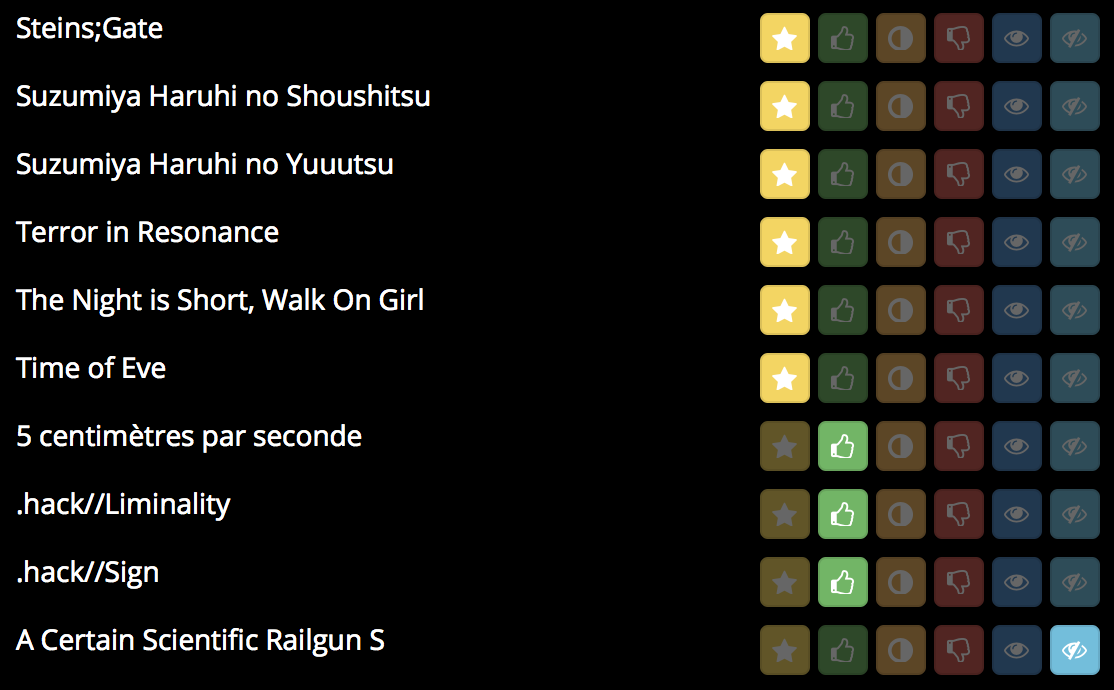
Mangaki prioritizes your watchlist
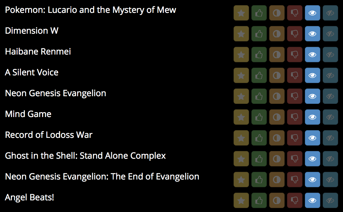
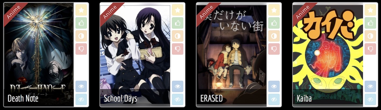
Browse the rankings: top works
>>> from mangaki.models import Work
>>> Work.objects.filter(category__slug='anime').top()[:8]
Why nonprofit?
- Why should blockbusters get all the fun/clicks/money?
- Maybe there is one precious, unknown anime \alert{for you}
- and we can help you find it
Driven by passion, not profit
- Everything is open source: \alert{github.com/mangaki}
- Python (Django), Vue.js
- Many Jupyter notebooks (check ‘em out!)
Awards: Microsoft Prize (2014) Japan Foundation (2016)
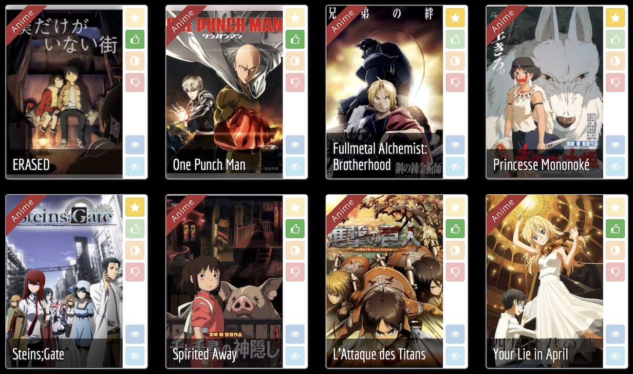
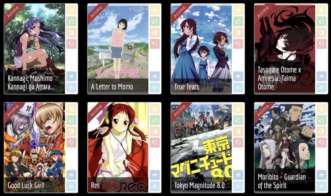
A simple idea: precious pearls
Work.objects.filter(category__slug='anime').pearls()[:8]
Recommender Systems
Problem
- Every user rates few items (1 %)
- How to infer missing ratings?
Example
\begin{tabular}{ccccc}
& \includegraphics[height=2.5cm]{figures/1.jpg} & \includegraphics[height=2.5cm]{figures/2.jpg} & \includegraphics[height=2.5cm]{figures/3.jpg} & \includegraphics[height=2.5cm]{figures/4.jpg}
Sacha & ? & 5 & 2 & ?
Ondine & 4 & 1 & ? & 5
Pierre & 3 & 3 & 1 & 4
Joëlle & 5 & ? & 2 & ?
\end{tabular}
Recommender Systems
Problem
- Every user rates few items (1 %)
- How to infer missing ratings?
Example
\begin{tabular}{ccccc}
& \includegraphics[height=2.5cm]{figures/1.jpg} & \includegraphics[height=2.5cm]{figures/2.jpg} & \includegraphics[height=2.5cm]{figures/3.jpg} & \includegraphics[height=2.5cm]{figures/4.jpg}
Sacha & \alert{3} & 5 & 2 & \alert{2}
Ondine & 4 & 1 & \alert{4} & 5
Pierre & 3 & 3 & 1 & 4
Joëlle & 5 & \alert{2} & 2 & \alert{5}
\end{tabular}
What is a machine learning algorithm?
Fit
\begin{center}
\begin{tabular}{ccc} \toprule
Ondine & \alert{like} & \emph{Zootopia}
Ondine & \alert{favorite} & \emph{Porco Rosso}
Sacha & \alert{favorite} & \emph{Tokikake}
Sacha & \alert{dislike} & \emph{The Martian}\ \bottomrule
\end{tabular}
\end{center}
Predict
\begin{center}
\begin{tabular}{ccc} \toprule
Ondine & \alert{\only<1>{?}\only<2>{favorite}} & \emph{The Martian}
Sacha & \alert{\only<1>{?}\only<2>{like}} & \emph{Zootopia}\ \bottomrule
\end{tabular}
\end{center}
What is a \alert{bad} machine learning algorithm?
Fit
\begin{center}
\begin{tabular}{ccc} \toprule
Ondine & \alert{like} & \emph{Zootopia}
Ondine & \alert{favorite} & \emph{Porco Rosso}
Sacha & \alert{favorite} & \emph{Tokikake}
Sacha & \alert{dislike} & \emph{The Martian}\ \bottomrule
\end{tabular}
\end{center}
\hfill 100% correct
Predict
\begin{center}
\begin{tabular}{ccc} \toprule
Ondine & \alert{dislike} & \emph{The Martian} (was: favorite)
Sacha & \alert{neutral} & \emph{Zootopia} (was: like)\ \bottomrule
\end{tabular}
\end{center}
\hfill 20% correct
Cannot generalize
What is a \alert{good} machine learning algorithm?
Fit
\begin{center}
\begin{tabular}{ccc} \toprule
Ondine & \alert{favorite} & \emph{Zootopia} (was: like)
Ondine & \alert{favorite} & \emph{Porco Rosso}
Sacha & \alert{favorite} & \emph{Tokikake}
Sacha & \alert{dislike} & \emph{The Martian}\ \bottomrule
\end{tabular}
\end{center}
\hfill 90% correct
Predict
\begin{center}
\begin{tabular}{ccc} \toprule
Ondine & \alert{like} & \emph{The Martian} (was: favorite)
Sacha & \alert{favorite} & \emph{Zootopia} (was: like)\ \bottomrule
\end{tabular}
\end{center}
\hfill 90% correct
How to compare algorithms?
\centering
\begin{tabular}{cccccc}
dislike & wontsee & neutral & willsee & like & favorite
-2 & -0.5 & 0.1 & 0.5 & 2 & 4
\end{tabular}
\raggedright
Penalty
- If I predict:
-
\alert{favorite} for favorite $\rightarrow$ 0 error
\alert{dislike} for favorite $\rightarrow$ $(4 - (-2))^2 = 36$ error
\alert{like} for favorite $\rightarrow$ 4 error
Error: Mean value of (difference)²
RMSE: square root of that
\alert<2>{Divide} / \alert<3,5>{Fit} / \alert<4,6>{Predict}
\begin{tabular}{c|c|c|c|c}
A likes 1 & & C likes 1 & & E \alert<3-4>{\only<3>{?}\only<1-2,4-6>{neutral}} 3
B likes 2 & B dislikes 3 & C likes 2 & D \alert<5-6>{\only<5>{?}\only<1-4,6>{wontsee}} 3 & C \alert<3-4>{\only<3>{?}\only<1-2,4-6>{willsee}} 2
& B likes 4 & & D \alert<5-6>{\only<5>{?}\only<1-4,6>{wontsee}} 4
\end{tabular}
Matrix factorization $\rightarrow$ reduce dimension to generalize
Idea: Do \alert{user2vec} for all users, \alert{item2vec} for all movies
such that users like movies that are in their direction.
Fit
- $R$ ratings, \alert{$U$} user vectors, \alert{$W$} work vectors.
\pause
Predict: Will user $i$ like item $j$?
- Just compute $\alert{U_i} \cdot \alert{W_j}$ and you will find out!
Algorithm \alert{ALS}: Alternating Least Squares (Zhou, 2008)
- Until convergence (~ 20 iterations):
- Fix $U$ (users) learn $W$ (works)
\hfill in order to minimize the error (+ something) - Fix $W$ find $U$
- Fix $U$ (users) learn $W$ (works)
Illustration of ALS
\only<1>{\includegraphics{figures/embed0.pdf}}
\only<2>{\includegraphics{figures/embed1.pdf}} \only<3>{\includegraphics{figures/embed2.pdf}} \only<4>{\includegraphics{figures/embed3.pdf}} \only<5>{\includegraphics{figures/embed4.pdf}} \only<6>{\includegraphics{figures/embed5.pdf}} \only<7>{\includegraphics{figures/embed6.pdf}} \only<8>{\includegraphics{figures/embed7.pdf}} \only<9>{\includegraphics{figures/embed8.pdf}} \only<10>{\includegraphics{figures/embed9.pdf}} \only<11>{\includegraphics{figures/embed10.pdf}} \only<12>{\includegraphics{figures/embed11.pdf}} \only<13>{\includegraphics{figures/embed12.pdf}} \only<14>{\includegraphics{figures/embed13.pdf}} \only<15>{\includegraphics{figures/embed14.pdf}} \only<16>{\includegraphics{figures/embed15.pdf}} \only<17>{\includegraphics{figures/embed16.pdf}} \only<18>{\includegraphics{figures/embed17.pdf}} \only<19>{\includegraphics{figures/embed18.pdf}} \only<20>{\includegraphics{figures/embed19.pdf}} \only<21>{\includegraphics{figures/embed20.pdf}} \only<22>{\includegraphics{figures/embed21.pdf}} \only<23>{\includegraphics{figures/embed22.pdf}} \only<24>{\includegraphics{figures/embed23.pdf}} \only<25>{\includegraphics{figures/embed24.pdf}} \only<26>{\includegraphics{figures/embed25.pdf}} \only<27>{\includegraphics{figures/embed26.pdf}} \only<28>{\includegraphics{figures/embed27.pdf}} \only<29>{\includegraphics{figures/embed28.pdf}} \only<30>{\includegraphics{figures/embed29.pdf}} \only<31>{\includegraphics{figures/embed30.pdf}} \only<32>{\includegraphics{figures/embed31.pdf}} \only<33>{\includegraphics{figures/embed32.pdf}} \only<34>{\includegraphics{figures/embed33.pdf}} \only<35>{\includegraphics{figures/embed34.pdf}} \only<36>{\includegraphics{figures/embed35.pdf}} \only<37>{\includegraphics{figures/embed36.pdf}} \only<38>{\includegraphics{figures/embed37.pdf}}
\only<39>{\includegraphics{figures/embed38.pdf}}
Why \alert{+ something}? Regularize to generalize
\begin{columns}
\begin{column}{0.6\linewidth}
Just minimize RMSE
May not be optimal\\vspace{2cm}
Minimize RMSE + regularization:
$\Rightarrow$ easier to optimize
\end{column}
\begin{column}{0.4\linewidth}
\hfill \includegraphics[width=\linewidth]{figures/nonreg.pdf}
\hfill \includegraphics[width=\linewidth]{figures/reg.pdf}
\end{column}
\end{columns}
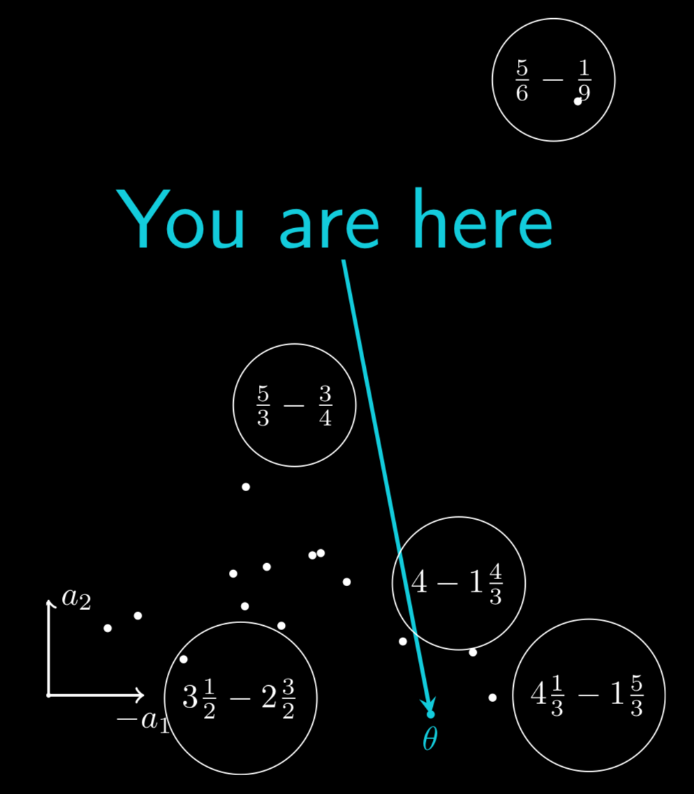
Visualizing all anime
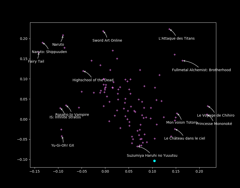 \
\
You will \alert{like} anime that are \alert{in your direction}
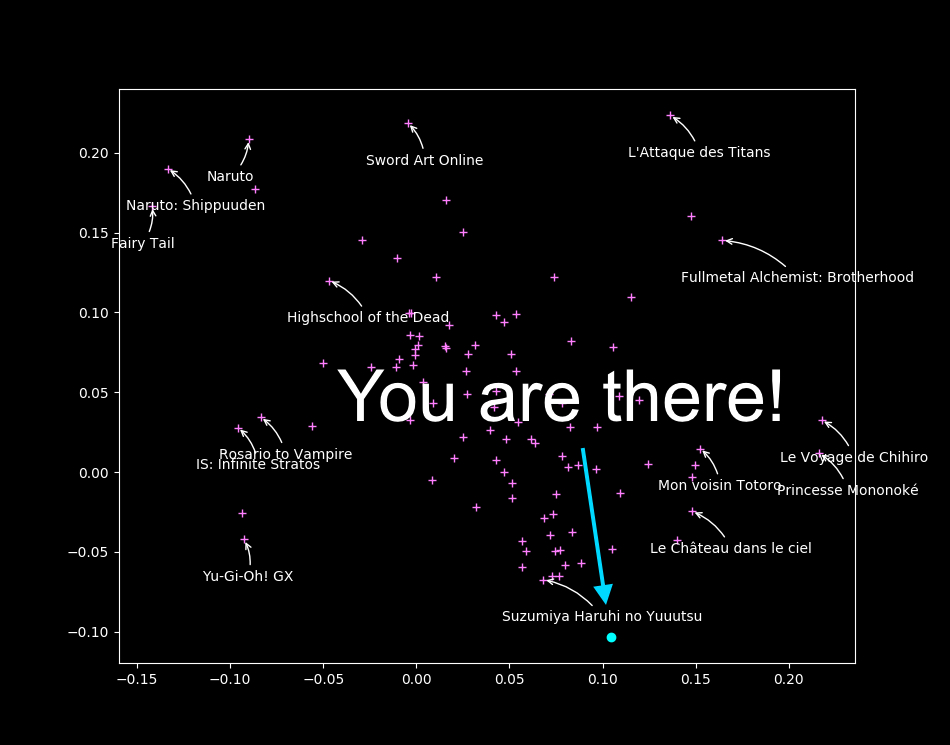 \
\
What did we do, precisely?
Newton’s method
To find the zeroes of $f : \mathbf{R} \to \mathbf{R}$:
\[x_{n + 1} = x_n - \frac{f(x_n)}{f'(x_n)}\]Optimization
What if we want to minimize $\mathcal{L}: \mathbf{R}^n \to \mathbf{R}$?
\[x_{n + 1} = x_n - {\underbrace{H\mathcal{L}(x_n)}_{n \times n \textnormal{ matrix}}}^{-1} \nabla \mathcal{L}(x_n)\]What if it is costly?
\[x_{n + 1} = x_n - \gamma \nabla \mathcal{L}(x_n)\]Oh, we just invented gradient descent.
Alternating Least Squares
| find \alert{$U_k$} that minimizes $$f(U_k) = \sum_{i, j} (\underbrace{\alert{U_i} \cdot W_j}{pred} - \underbrace{r{ij}}_{real})^2 + \underbrace{\lambda | \alert{U_i} | _2^2 + \lambda | W_j | 2^2}{regularization}$$ |
(by the way: the derivative of $\alert{u} \cdot v$ with respect to $\alert{u}$ is $v$)
\pause
find the zeroes of \(f'(U_k) = \sum_{j \textnormal{ rated by } k} 2 (\alert{U_k} \cdot W_j - r_{kj}) W_j + 2 \lambda \alert{U_k} = 0\) can be rewritten $A\alert{U_k} = B$ so $\alert{U_k} = A^{-1}B$ (easy!)
Complexity: $O(n^3)$ where $n$ is the number of items rated by $U_k$
Stochastic Gradient Descent
\[U_k \leftarrow U_k - \gamma f'(U_k)\] \[U_k \leftarrow (1 - 2 \gamma \lambda) U_k - 2 \gamma \sum_{j \textnormal{ rated by } k} \underbrace{(U_k \cdot W_j - r_{kj})}_{\textnormal{prediction error}} W_j\]$U_k$ is updated according to its neighbors $W_j$
Benchmarks
ALS: minimizing $U$ then $W$ then $U$ then $W$
SGD: minimizing $U$ and $W$ at the same time
\centering
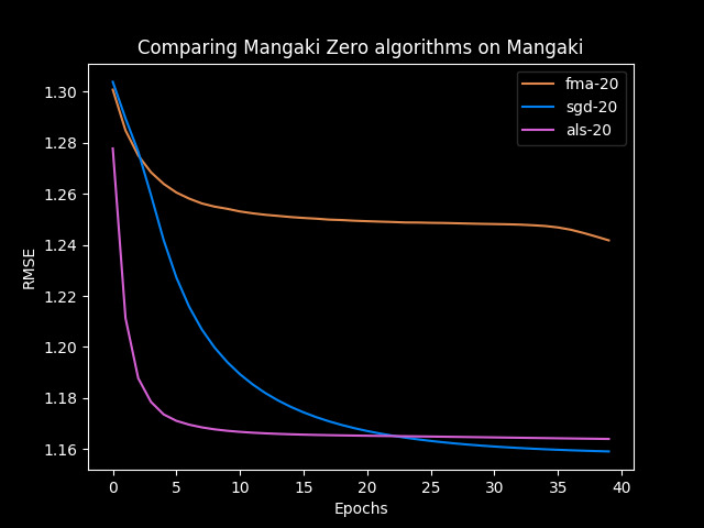 {width=84%}\
Drawback with collaborative filtering
Issue: Item Cold-Start
- If no ratings are available for a work $j$
$\Rightarrow$ Its vector $W_j$ cannot be learned :-(
No way to distinguish between unrated works.
But we have (many) posters!
II – Factorization Machines
Learning multidimensional feature embeddings
Logistic Regression
Learn a \alert{bias} for each feature (each user, item, etc.)
Factorization Machines
Learn a \alert{bias} and an \alert{embedding} for each feature
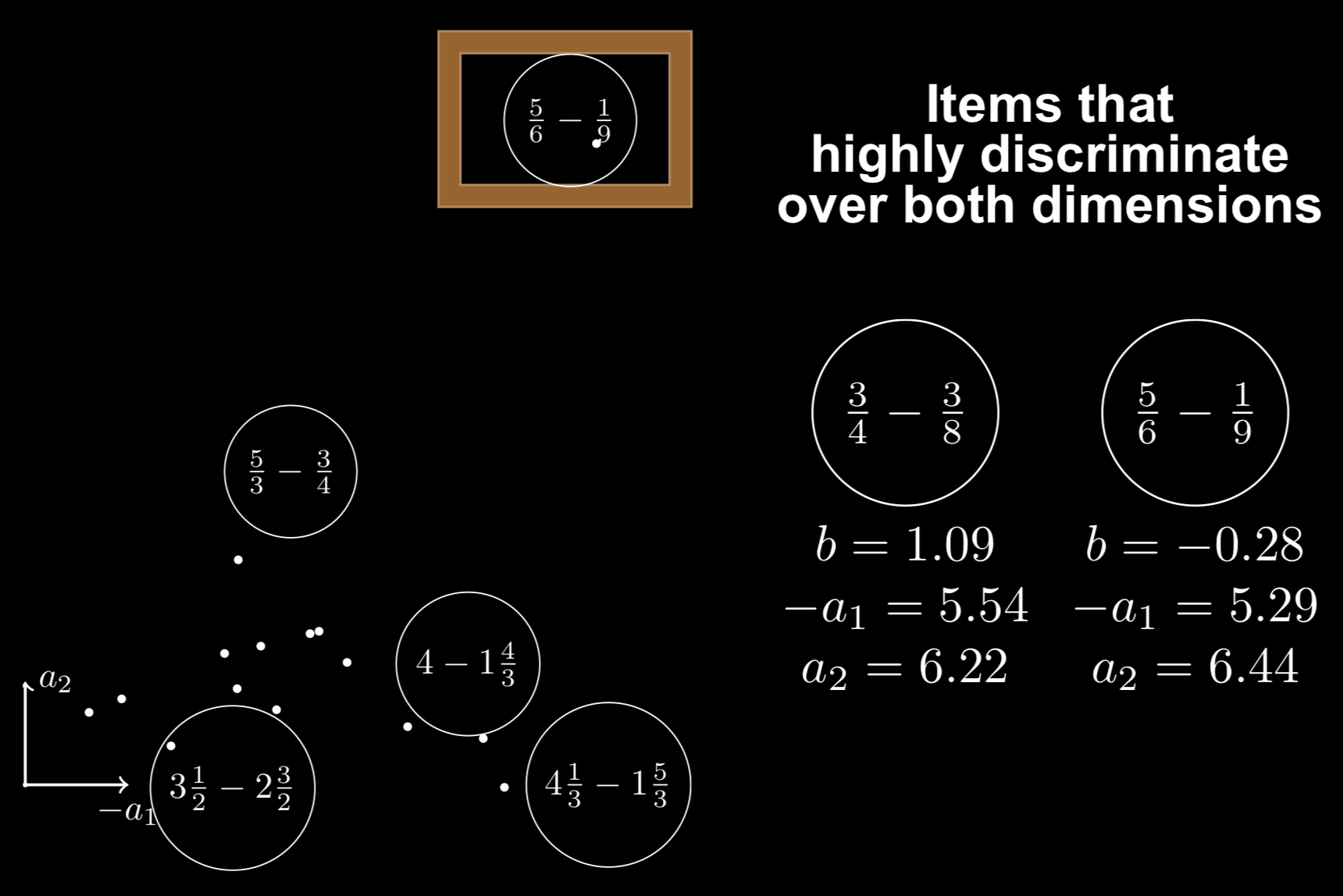
What can be done with multidimensional embeddings?
\centering
 {width=60%}
Interpreting the components
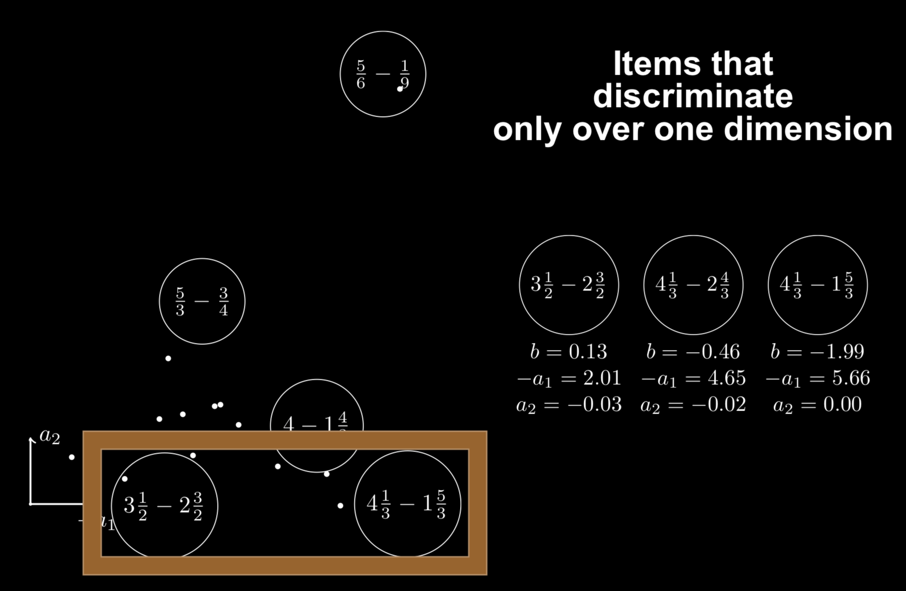
Interpreting the components
How to model pairwise interactions with side information?
If you know user $i$ watched item $j$ on \alert{TV} (not theatre)
How to model it?
$y$: rating of user $i$ over item $j$
Biases
\[y = \theta_i + e_j\]Collaborative filtering
\[y = \theta_i + e_j + \langle \bm{v_\textnormal{user $i$}}, \bm{v_\textnormal{item $j$}} \rangle\]\pause
With side information
\small \vspace{-3mm} \(y = \theta_i + e_j + \alert{w_\textnormal{TV}} + \langle \bm{v_\textnormal{user $i$}}, \bm{v_\textnormal{item $j$}} \rangle + \langle \bm{v_\textnormal{user $i$}}, \alert{\bm{v_\textnormal{TV}}} \rangle + \langle \bm{v_\textnormal{item $j$}}, \alert{\bm{v_\textnormal{TV}}} \rangle\)
Factorization Machines
Just pick features (ex. user, item, skill) and you get a model
Each feature $k$ is modeled by bias $\alert{w_k}$ and embedding $\alert{\bm{v_k}}$.\vspace{2mm} \begin{columns} \begin{column}{0.47\linewidth} \includegraphics[width=\linewidth]{figures/fm-rv.png} \end{column} \begin{column}{0.53\linewidth} \includegraphics[width=\linewidth]{figures/fm2-rv.png} \end{column} \end{columns}\vspace{-2mm}
\hfill $\logit p(\bm{x}) = \mu + \underbrace{\sum_{k = 1}^N \alert{w_k} x_k}\textnormal{logistic regression} + \underbrace{\sum{1 \leq k < l \leq N} x_k x_l \langle \alert{\bm{v_k}}, \alert{\bm{v_l}} \rangle}_\textnormal{pairwise relationships}$
\small \fullcite{KTM2019}
Regression with sparse features (very elegant!)
$\bm{x}$ concatenation of one-hot vectors \only<3->{(ex. at positions $s$ and $t$)}
$\langle \bm{w}, \bm{x} \rangle = \sum_i w_i x_i \only<3->{= w_s + w_t}$
| $ | V\bm{x} | ^2 = \sum_{\alert{i, j}} x_i x_j \langle \bm{v}_i, \bm{v}_j \rangle \geq 0$ |
\pause
| $\frac12 ( | V\bm{x} | ^2 - \mathbf{1}^T (V \circ V) (\bm{x} \circ \bm{x})) = \sum_{\alert{i < j}} x_i x_j \langle \bm{v}_i, \bm{v}_j \rangle \only<3->{= \langle \bm{v}_s, \bm{v}_t \rangle}$ |
\pause \pause
Factorization machines (Rendle 2012)
$P(\langle \bm{x}, \bm{v}_i \rangle)$ for a polynomial $P$
The Blondel Trilogy
- Polynomial networks and FMs (ICML 2016)
- Multi-output polynomial networks and FMs (NIPS 2017)
- Higher-order FMs (NIPS 2016)
III – Binary factorization
Chess players have Elo ratings
Elo ratings are updated after each match
If player 1 (550) beats player 2 (600)
Then player 1 will $\uparrow$ (560) and player 2 will $\downarrow$ (590)
Let’s ask Harvard students
\centering
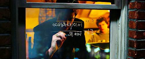
(The Social Network)
Let’s ask Harvard students
\centering
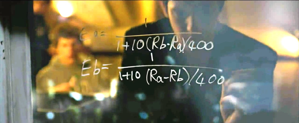
(The Social Network)
K-Factor???
\centering
(Not The Social Network)
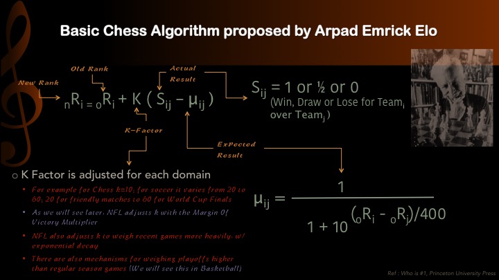
Old models still used today
Elo (1960–1978)
\[P(\theta_i \textnormal{ beats } \theta_j) = \frac1{1 + 10^{(\theta_j - \theta_i)/400}}\]Item response theory (1960)
\[P(\theta_i \textnormal{ solves } d_j) = \frac1{1 + e^{-(\theta_i - d_j)}}\]Examples
Used in PISA, GMAT, Pix.
Maximum likelihood estimation
Given outcomes $r \in {0, 1}$, how to estimate $\theta$?
$p = \frac1{1 + e^{-(\theta - d)}} = \sigma(\theta - d)$
Thanks to logistic function: $p’ = p(1 - p)$
$L(\theta) = \log p^r (1 - p)^{1 - r} = r \log p + (1 - r) \log (1 - p)$
$\nabla_\theta L = \frac{\partial L}{\partial \theta} = r - p$
$\theta_{t + 1} = \theta_t + \gamma \underbrace{\nabla_\theta L}_{r - p}$
\pause
Thus it is \alert{online gradient ascent}! K-factor = $\gamma$ = learning rate.\bigskip
The chess statistician Jeff Sonas believes that the original $K=10$ value (for players rated above 2400) is inaccurate in Elo’s work.
Evolving over time
Players ability increase as they win matches over other players
So players may have an optimistic strategy to plan their matches
Factorization: learning vectors
From some $R_{ij}$ infer other $R_{ij}$
Collaborative filtering
Learn model $U, V$ such that $R \simeq UV \quad \widehat{r_{ij}} = \langle \bm{u}i, \bm{v}_j \rangle$
Optimize regularized least squares $\sum{i, j} (\widehat{r_{ij}} - r_{ij})^2 + \lambda (||U||^2_F + ||V||^2_F)$
Binary version
Learn model $U, V$ such that $R \simeq \sigma(UV) \quad \widehat{r_{ij}} = \sigma(\langle \bm{u}_i, \bm{v}_j \rangle)$ Optimize likelihood
EM algorithm via MCMC: sample $U$, optimize $V$ (Cai, 2010)
Slow, $d \leq 6$
Scaling to big data
Gradient descent
For each example update parameters
\pause
Batch gradient descent
Compute the gradient on all examples and update parameters
\pause
Stochastic gradient descent
Sample examples and update parameters
\pause
Minibatch gradient descent
Sample a minibatch of examples and update parameters
Scaling to high dimension
$\theta_{t + 1} = \theta_t - \gamma \nabla_\theta \mathcal{L} \Rightarrow$ Replace $\nabla_\theta \mathcal{L}$ with an unbiased estimate $\tilde\nabla_\theta \mathcal{L}$ \centering \includegraphics[width=0.98\linewidth]{figures/cfirt-rv.png}
IV – Deep Factorization
Drawback with collaborative filtering
Issue: Item Cold-Start
- If no ratings are available for a work $j$
$\Rightarrow$ Its vector $W_j$ cannot be learned :-(
No way to distinguish between unrated works.
But we have (many) posters!
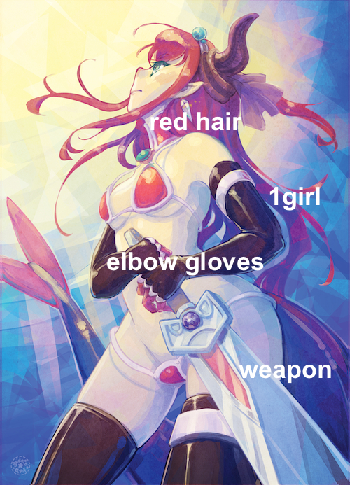
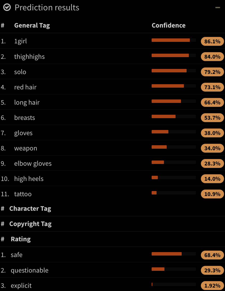
Illustration2Vec (Saito and Matsui, 2015)
\centering
 {height=70%}\
 {height=70%}\
- CNN (VGG-16) pretrained on ImageNet (photos)
- Retrained on Danbooru (1.5M manga illustrations with tags)
- 502 most frequent tags kept, outputs \alert{tag weights}
LASSO for sparse linear regression
$T$ matrix of 15000 works $\times$ 502 tags ($T_j$: tags of work $j$)
Fit
- Each user is described by its preferences over tags \alert{$P_i$}
- \alert{LASSO constraint}: user likes/hates few tags
- Learn user preferences \alert{$P_i$} such that \(\hat{r}_{ij}^{LASSO} = \alert{P_i} \cdot T_j.\)
\pause
Predict: Will user $i$ like work $j$?
- Here is a new work with a poster and tags $T_j$
- Just compute $\alert{P_i} \cdot T_j$ and you will find out!
Interpretation and explanation of user preferences
- You seem to like \alert{\emph{magical girls}} but not \alert{\emph{blonde hair}}
$\Rightarrow$ Look! All of them are \alert{\emph{brown hair}}! Buy now!
Combine models
Which model should we choose between ALS and LASSO?
- Answer
-
Both!
- Methods
-
boosting, bagging, model stacking, blending.
- Idea
-
find $\alert<2>{\alpha\only<2>{j}}$ s.t. $\hat{r{ij}} \triangleq \alert<2>{\alpha\only<2>{j}} \hat{r}{ij}^{ALS} + (1 - \alert<2>{\alpha\only<2>{j}}) \hat{r}{ij}^{LASSO}.$
If popular, listen to ALS more than LASSO
Our Architecture
\includegraphics{figures/archiwhite-rv.pdf}
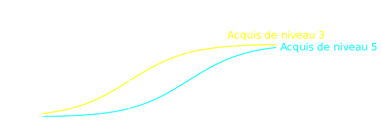
Examples of $\alpha_j$
\centering \includegraphics{figures/curve1-rv.pdf}
Mimics ALS \(\hat{r_{ij}} \triangleq \alert1 \hat{r}_{ij}^{ALS} + \alert0 \hat{r}_{ij}^{LASSO}.\)
Examples of $\alpha_j$
\centering \includegraphics{figures/curve2-rv.pdf}
Mimics LASSO \(\hat{r_{ij}} \triangleq \alert0 \hat{r}_{ij}^{ALS} + \alert1 \hat{r}_{ij}^{LASSO}.\)
Examples of $\alpha_j$
\centering \includegraphics{figures/curve3-rv.pdf} \(\hat{r}_{ij}^{BALSE} = \begin{cases} \hat{r}_{ij}^{ALS} & \text{if item $j$ was rated at least $\gamma$ times}\\ \hat{r}_{ij}^{LASSO} & \text{otherwise} \end{cases}\) But we can’t: \alert{Not differentiable!}
Examples of $\alpha_j$
\centering \includegraphics{figures/curve4-rv.pdf} \(\hat{r}_{ij}^{BALSE} = \alert{\sigma(\beta(R_j - \gamma))} \hat{r}_{ij}^{ALS} + \left(1 - \alert{\sigma(\beta(R_j - \gamma))}\right) \hat{r}_{ij}^{LASSO}\) $\beta$ and $\gamma$ are learned by stochastic gradient descent.
Blended Alternate Least Squares with Explanation
\centering
Blended Alternate Least Squares with Explanation
Blended Alternate Least Squares with Explanation
Blended Alternate Least Squares with Explanation
Blended Alternate Least Squares with Explanation
Blended Alternate Least Squares with Explanation
Blended Alternate Least Squares with Explanation \only<2>{(\alert{BALSE})}
Comparing algorithms: cross-validation
- 80% of the ratings are used for training
- 20% of the ratings are kept for testing
Different sets of items:
- Whole test set of works
- 1000 works least rated (1.5%)
- Cold-start: works not seen in the training set (only the posters)
Results
\centering
\
Summing up
We presented BALSE, a model that:
- uses information in the \alert{ratings} (collaborative filtering)
- uses information in the \alert{posters} using CNNs (content-based)
- combine them in a \alert{nonlinear} way
to \alert{improve} the recommendations, and \alert{explain} them.
Future work: Make your neural network watch the anime
Extract frames from episodes

\hfill \emph{Cowboy Bebop EP 23} “Brain Scratch”, Sunrise
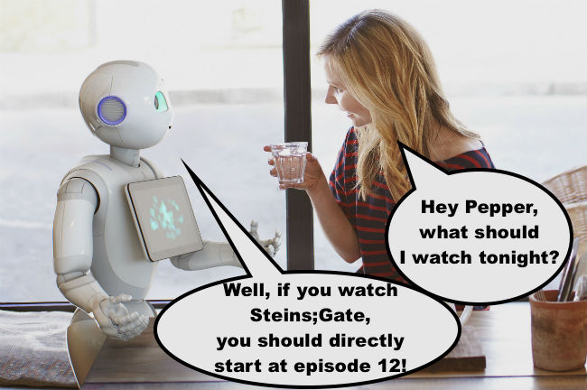
Coming soon: Watching assistant
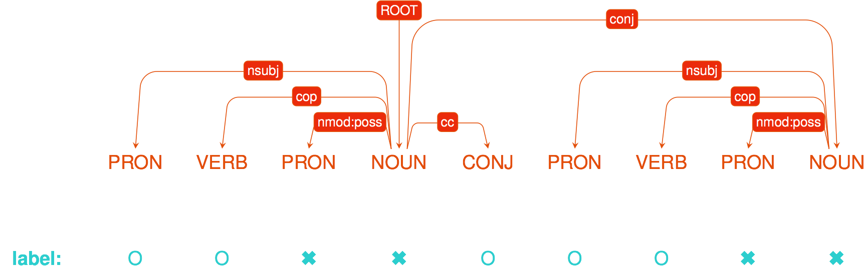
Deep Factorization Machines
Learn layers \alert{$W^{(\ell)}$} and \alert{$b^{(\ell)}$} such that: \(\begin{aligned}[c] \bm{a}^{0}(\bm{x}) & = (\alert{\bm{v_{\texttt{user}}}}, \alert{\bm{v_{\texttt{item}}}}, \alert{\bm{v_{\texttt{skill}}}}, \ldots)\\ \bm{a}^{(\ell + 1)}(\bm{x}) & = \ReLU(\alert{W^{(\ell)}} \bm{a}^{(\ell)}(\bm{x}) + \alert{\bm{b}^{(\ell)}}) \quad \ell = 0, \ldots, L - 1\\ y_{DNN}(\bm{x}) & = \ReLU(\alert{W^{(L)}} \bm{a}^{(L)}(\bm{x}) + \alert{\bm{b}^{(L)}}) \end{aligned}\)
\[\logit p(\bm{x}) = y_{FM}(\bm{x}) + y_{DNN}(\bm{x})\]\fullcite{Duolingo2018}
Comparison
- FM: $y_{FM}$ factorization machine with $\lambda = 0.01$
- Deep: $y_{DNN}$: multilayer perceptron
- DeepFM: $y_{DNN} + y_{FM}$ with shared embedding
- Bayesian FM: $\alert{w_k}, \alert{v_{kf}} \sim \mathcal{N}(\alert{\mu_f}, 1/\alert{\lambda_f})$
$\alert{\mu_f} \sim \mathcal{N}(0, 1)$, $\alert{\lambda_f} \sim \Gamma(1, 1)$ (trained using Gibbs sampling)
Various types of side information
- first:
<discrete>(user,token,countries, etc.) - last:
<discrete>+<continuous>(time+days) - pfa:
<discrete>+wins+fails
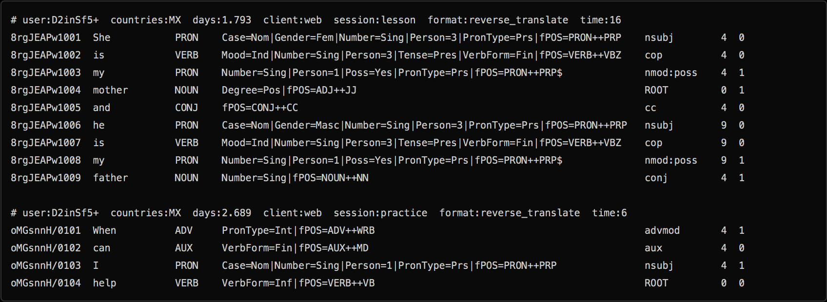
Duolingo dataset
Results
\small
\begin{tabular}{cccccccc}
\toprule
Model & $d$ & epoch & train & first & last & pfa
\midrule
Bayesian FM & 20 & 500/500 & – & 0.822 & – & –
Bayesian FM & 20 & 500/500 & – & – & 0.817 & –
DeepFM & 20 & 15/1000 & 0.872 & 0.814 & – & –
Bayesian FM & 20 & 100/100 & – & – & 0.813 & –
FM & 20 & 20/1000 & 0.874 & 0.811 & – & –
Bayesian FM & 20 & 500/500 & – & – & – & 0.806
FM & 20 & 21/1000 & 0.884 & – & – & 0.805
FM & 20 & 37/1000 & 0.885 & – & 0.8 & –
DeepFM & 20 & 77/1000 & 0.89 & – & 0.792 & –
Deep & 20 & 7/1000 & 0.826 & 0.791 & – & –
Deep & 20 & 321/1000 & 0.826 & – & 0.79 & –
LR & 0 & 50/50 & – & – & – & 0.789
LR & 0 & 50/50 & – & 0.783 & – & –
LR & 0 & 50/50 & – & – & 0.783 & –
\bottomrule
\end{tabular}
Duolingo ranking
\centering
\begin{tabular}{cccc} \toprule
Rank & Team & Algo & AUC\ \midrule
1 & SanaLabs & RNN + GBDT & .857
2 & singsound & RNN & .854
2 & NYU & GBDT & .854
4 & CECL & LR + L1 (13M feat.) & .843
5 & TMU & RNN & .839\ \midrule
7 (off) & JJV & Bayesian FM & .822
8 (off) & JJV & DeepFM & .814
10 & JJV & DeepFM & .809\ \midrule
15 & Duolingo & LR & .771\ \bottomrule
\end{tabular}
\raggedright \small \fullcite{Settles2018}
Thank you! \hfill jill-jenn.vie@inria.fr
Try our recommender system: \alert{mangaki.fr}
\raggedright
\pause
Any questions?
Know more
- AI for Manga & Anime: \alert{research.mangaki.fr}
\centering \includegraphics[height=3cm]{figures/styletransfer.jpg}