Jill-Jênn Vie
Researcher at Inria
% Embeddings: learning representations for unsupervised learning % Marc Lelarge; Kevin Scaman; Jill-Jênn Vie % Oct 28, 2022 — aspectratio: 169 header-includes: |
  \usepackage{tikz}
  \usepackage{bm}
  \def\x}
  \def\y}
  \def\u}
  \def\v}
  \def\X}
  \def\e}
  \def\W}
  \def\L{\mathcal{L}}
  \def\R{\mathbf{R}}
  \usepackage{datetime2}
Supervised learning \hfill Unsupervised learning
:::::: {.columns} ::: {.column} We observe $\x, y$
i.e. classification, regression
 :::
::: {.column}
\pause
We just observe $\x$
:::
::: {.column}
\pause
We just observe $\x$
i.e. raw text, music, ratings
 :::
::::::
:::
::::::
\pause
It all deals with learning a representation of the data: embedding entities into $\R^d$
Context
- Dealing with unlabeled data, like raw text
- Dealing with tabular data, which mixes \alert{categorical} and continuous variables
- Detecting outliers in the dataset
- Or mistakes in labels
Natural language processing
- A document can be represented as a sparse vector $\x$ of size 60,000 where $\x_i$ is the number of occurrences of the $i$th word.
- Could we guess meaning from context like humans?
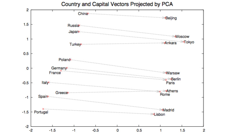
Learned embeddings have interesting properties: word2vec
\centering
 {width=70%}
\raggedright \small \fullcite{mikolov2013}
Multilingual word embeddings (unsupervised)
\centering

 {width=40%}
\raggedright \fullcite{lample2018word}
Application: Recommender Systems
Problem
- Every user rates few items (1 %)
- How to infer missing ratings?
Example
\begin{tabular}{ccccc}
& \includegraphics[height=2.5cm]{figures/1.jpg} & \includegraphics[height=2.5cm]{figures/2.jpg} & \includegraphics[height=2.5cm]{figures/3.jpg} & \includegraphics[height=2.5cm]{figures/4.jpg}
Sacha & ? & 5 & 2 & ?
Ondine & 4 & 1 & ? & 5
Pierre & 3 & 3 & 1 & 4
Joëlle & 5 & ? & 2 & ?
\end{tabular}
Application: Recommender Systems
Problem
- Every user rates few items (1 %)
- How to infer missing ratings?
Example
\begin{tabular}{ccccc}
& \includegraphics[height=2.5cm]{figures/1.jpg} & \includegraphics[height=2.5cm]{figures/2.jpg} & \includegraphics[height=2.5cm]{figures/3.jpg} & \includegraphics[height=2.5cm]{figures/4.jpg}
Sacha & \alert{3} & 5 & 2 & \alert{2}
Ondine & 4 & 1 & \alert{4} & 5
Pierre & 3 & 3 & 1 & 4
Joëlle & 5 & \alert{2} & 2 & \alert{5}
\end{tabular}
Encoding the problem
Matrix completion (unsupervised)
Given sparse entries $M_{ij}$ find the other entries $M_{ij}$
Supervised problem
- $\X = {(i, j)}$ are the categorical observed indices (ex. user $i$ and item $j$)
- $\y = {R_{ij}}$ are the continuous (or categorical) ratings
Learning embeddings
Embedding $n$ entities into $\R^d$ is equivalent to learning a $n \times d$ matrix $\W$ s.t. embedding of entity $i$ is $W_i$.
- One-hot encoding
- $\e_j = (0, \ldots, 0, \underbrace1_j, 0, \ldots, 0)$ so that $\W \e_j = W_j$
\centering
Dimensionality reduction, or best approximation of rank $k$
Input: $n \times m$ matrix $\X$
| Minimize: $ | \X - M | ^22 = \sum{i, j} (X_{ij} - M_{ij})^2$ where $rank(M) = k$ |
\pause
Solution: compute the singular value decomposition (SVD) $\X = U \Sigma V^T$ where
- $U$ ($n \times r$) is orthogonal: $U^T U = I_r$ where $r = rank(\X)$
- $\Sigma$ ($r \times r$) is diagonal: its values $\lambda_1 \geq \ldots \geq \lambda_r > 0$
- $V$ ($m \times r$) is orthogonal: $V^T V = I_r$
$k$-SVD is truncated to $k$ biggest singular values. $M = U_k \Sigma_k V_k^T$ is solution. And $W = U_k \Sigma_k$ is a $n \times k$ matrix of embeddings (pca.transform).
KNN $\rightarrow$ measure similarity between users (or items)
$K$-nearest neighbors
- $R_u$ represents the row vector of user $u$ in the rating matrix (users $\times$ items).
- Similarity score between users (cosine): \(score(u, v) = \frac{R_u \cdot R_v}{||R_u|| \cdot ||R_v||}.\)
- Let’s identify the $k$-nearest neighbors of user $u$
- And recommend to user $u$ what $u$’s neighbors liked, but $u$ didn’t watch
\pause
Hint
| If $R’$ the $N \times M$ matrix of rows $\frac{R_u}{ | R_u | }$, we can get the $N \times N$ score matrix by computing $R’ R’^T$. May not fit in memory. |
Matrix factorization $\rightarrow$ reduce dimension to generalize
\vspace{-7mm}
\(R = \left(\begin{array}{c} R_1\\ R_2\\ \vdots\\ R_n \end{array}\right) = \raisebox{-1cm}{\begin{tikzpicture} \draw (0,0) rectangle (2.5,2); \end{tikzpicture}} = \raisebox{-1cm}{\begin{tikzpicture} \draw (0,0) rectangle ++(1,2); \draw node at (0.5,1) {$U$}; \draw (1.1,1) rectangle ++(2.5,1); \draw node at (2.35,1.5) {$P$}; \end{tikzpicture}}\) \(\text{$R$: 600 users $\times$ 9k works} \iff \left\{\begin{array}{l} \text{$U$: 600 users $\times$ \alert{20 profiles}}\\ \text{$P$: \alert{20 profiles} $\times$ 9k works}\\ \end{array}\right.\) $\R_\text{Bob}$ is a linear combination of profiles $P_1$, $P_2$, etc.
\pause
Interpreting Key Profiles
\begin{tabular}{@{}lccc@{}}
If $P$ & $P_1$: adventure & $P_2$: romance & $P_3$: plot twist
And $U_{\textnormal{Bob}}$ & $0.2$ & $-0.5$ & $0.6$
\end{tabular}
$\Rightarrow$ Bob \alert{likes a bit} adventure, \alert{hates} romance, \alert{loves} plot twists.
Matrix factorization $\rightarrow$ reduce dimension to generalize
Train
- $R$ ratings, \alert{$U$} user embeddings, \alert{$V$} item embeddings.
\pause
Test: Will user $i’$ like item $j’$?
- Just compute $\u_{i’}^T \v_{j’}$
Objective: regularized squared loss
\[\L = \sum_{i,j}~(\underbrace{\u_i^T \v_j}_{\textnormal{pred}} - \underbrace{r_{ij}}_{\textnormal{real}})^2 + \underbrace{\lambda || \u_i ||_2^2 + \lambda || \v_j ||_2^2}_{\textnormal{regularization}}\]Variants
SVD: $\sum_{\textnormal{\alert{all} } i, j}~(\u_i^T \v_j - r_{ij})^2$ (missing pairs are imputed to zero)
ALS-WR : $\sum_{i, j \textnormal{\alert{ known}}}~(\u_i^T \v_j - r_{ij})^2 + \lambda (\sum_i N_i ||\u_i||^2 + \sum_j M_j ||\v_j||^2)$
where $N_i$ (resp. $M_j$): how many times user $i$ rated items (resp. item $j$ was rated)
Computing the gradients
\[\L = \sum_{i,j} (\underbrace{\u_i^T \v_j}_{\textnormal{pred}} - \underbrace{r_{ij}}_{\textnormal{real}})^2 + \underbrace{\lambda || \u_i ||_2^2 + \lambda || \v_j ||_2^2}_{\textnormal{regularization}}\]\pause
$\L$ is (polynomial and) convex in each $\u_k$ or $\v_\ell$.
Finding \alert{$\u_k$} that minimizes $\L$ $\Rightarrow$ Finding the zeroes of \(\frac{\partial \L}{\partial \u_k} = \sum_{j \textnormal{ rated by } k} 2 (\alert{\u_k}^T \v_j - r_{kj}) \v_j + 2 \lambda \alert{\u_k} = 0\) can be rewritten $A\alert{\u_k} = B$ so $\alert{\u_k} = A^{-1}B$ (closed form)
Complexity: $O(d^3)$ where $d$ is the (embedding) size of $A$ (but can be parallelized)
\pause
Algorithm \alert{ALS}: Alternating Least Squares (Zhou, 2008)
- Until convergence (few iterations):
- Fix $U$ (users) learn $V$ (items) in order to minimize $\L$
- Fix $V$ find $U$
Illustration of Alternating Least Squares
\only<1>{\includegraphics[width=0.9\linewidth]{figures/embed0.pdf}} \only<2>{\includegraphics[width=0.9\linewidth]{figures/embed1.pdf}} \only<3>{\includegraphics[width=0.9\linewidth]{figures/embed2.pdf}} \only<4>{\includegraphics[width=0.9\linewidth]{figures/embed3.pdf}} \only<5>{\includegraphics[width=0.9\linewidth]{figures/embed4.pdf}} \only<6>{\includegraphics[width=0.9\linewidth]{figures/embed5.pdf}} \only<7>{\includegraphics[width=0.9\linewidth]{figures/embed6.pdf}} \only<8>{\includegraphics[width=0.9\linewidth]{figures/embed7.pdf}} \only<9>{\includegraphics[width=0.9\linewidth]{figures/embed8.pdf}} \only<10>{\includegraphics[width=0.9\linewidth]{figures/embed9.pdf}} \only<11>{\includegraphics[width=0.9\linewidth]{figures/embed10.pdf}} \only<12>{\includegraphics[width=0.9\linewidth]{figures/embed11.pdf}} \only<13>{\includegraphics[width=0.9\linewidth]{figures/embed12.pdf}} \only<14>{\includegraphics[width=0.9\linewidth]{figures/embed13.pdf}} \only<15>{\includegraphics[width=0.9\linewidth]{figures/embed14.pdf}} \only<16>{\includegraphics[width=0.9\linewidth]{figures/embed15.pdf}} \only<17>{\includegraphics[width=0.9\linewidth]{figures/embed16.pdf}} \only<18>{\includegraphics[width=0.9\linewidth]{figures/embed17.pdf}} \only<19>{\includegraphics[width=0.9\linewidth]{figures/embed18.pdf}} \only<20>{\includegraphics[width=0.9\linewidth]{figures/embed19.pdf}} \only<21>{\includegraphics[width=0.9\linewidth]{figures/embed20.pdf}} \only<22>{\includegraphics[width=0.9\linewidth]{figures/embed21.pdf}} \only<23>{\includegraphics[width=0.9\linewidth]{figures/embed22.pdf}} \only<24>{\includegraphics[width=0.9\linewidth]{figures/embed23.pdf}} \only<25>{\includegraphics[width=0.9\linewidth]{figures/embed24.pdf}} \only<26>{\includegraphics[width=0.9\linewidth]{figures/embed25.pdf}} \only<27>{\includegraphics[width=0.9\linewidth]{figures/embed26.pdf}} \only<28>{\includegraphics[width=0.9\linewidth]{figures/embed27.pdf}} \only<29>{\includegraphics[width=0.9\linewidth]{figures/embed28.pdf}} \only<30>{\includegraphics[width=0.9\linewidth]{figures/embed29.pdf}} \only<31>{\includegraphics[width=0.9\linewidth]{figures/embed30.pdf}} \only<32>{\includegraphics[width=0.9\linewidth]{figures/embed31.pdf}} \only<33>{\includegraphics[width=0.9\linewidth]{figures/embed32.pdf}} \only<34>{\includegraphics[width=0.9\linewidth]{figures/embed33.pdf}} \only<35>{\includegraphics[width=0.9\linewidth]{figures/embed34.pdf}} \only<36>{\includegraphics[width=0.9\linewidth]{figures/embed35.pdf}} \only<37>{\includegraphics[width=0.9\linewidth]{figures/embed36.pdf}} \only<38>{\includegraphics[width=0.9\linewidth]{figures/embed37.pdf}} \only<39>{\includegraphics[width=0.9\linewidth]{figures/embed38.pdf}}
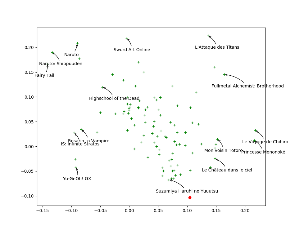
Close $\v_j$ mean similar movies
\centering
 {width=80%}
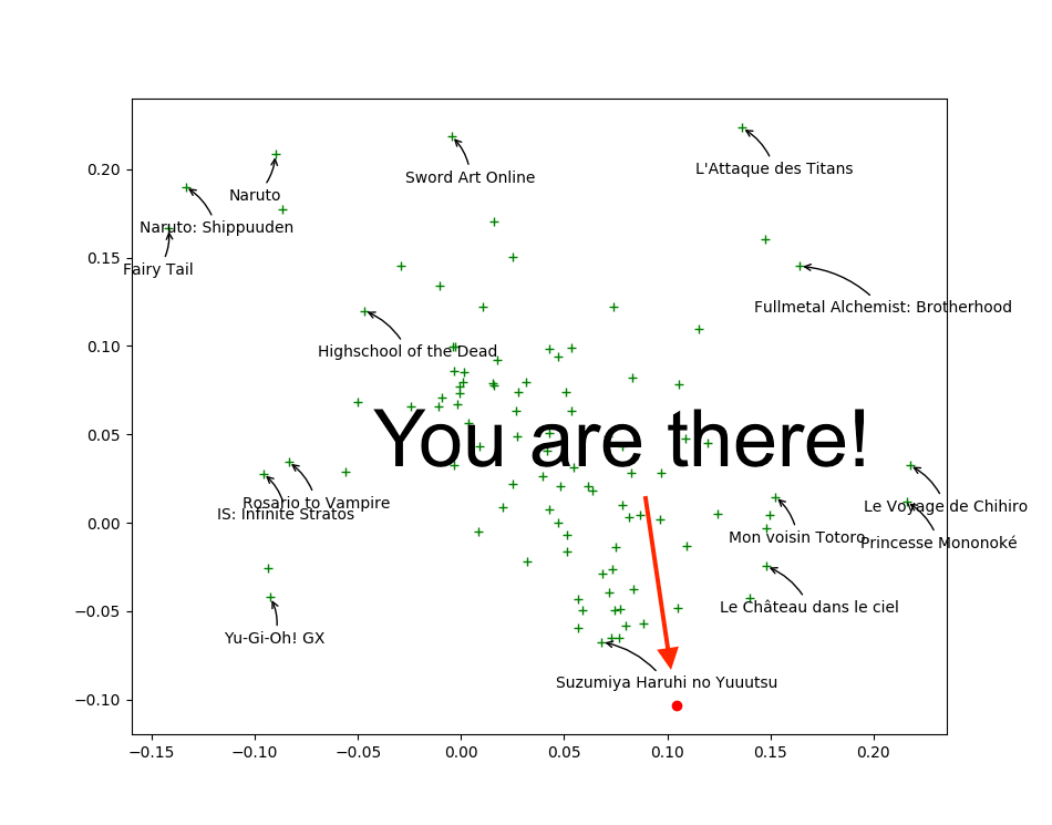
$\u_i$ will like movies in its direction
\centering
 {width=80%}
word2vec: the Skip-Gram model
We want, given a word $w \sim P(W)$, to predict its \alert{context} (i.e. the words around it).
Oh, it’s a classification problem! With 60,000 classes. \(P(c | w) = \textnormal{softmax}(\u_w^T \v_c) \propto \exp(\u_w^T \v_c)\)
Cross-entropy would look like: \(\L = \log \sigma(\u_w^T \v_c) + \sum_{\substack{i = 1\\c_i \neq c}}^{60000} \log (1 - \sigma(\u_w^T \v_{c_i}))\)
So instead let’s just sample $k$ words from vocabulary proportionally to their occurrence: \(\L = \sum_{w, c} \log \sigma(\u_w^T \v_c) + \sum_{\substack{i = 1\\c_i \sim P(W)}}^k \log (1 - \sigma(\u_w^T \v_{c_i}))\)
Neural Word Embedding as Implicit Matrix Factorization
Noise contrastive estimation
\vspace{-5mm} \(\L = \sum_{w, c} \log \sigma(\u_w^T \v_c) + \sum_{\substack{i = 1\\c_i \sim P(W)}}^k \log (1 - \sigma(\u_w^T \v_{c_i}))\)
Negative sampling (similar objective)
\vspace{-5mm} \(\L = \sum_{w, c} \log \sigma(\u_w^T \v_c) + \sum_{\substack{i = 1\\c_i \sim P(W)}}^k \log \sigma(-\u_w^T \v_{c_i}))\) This objective is equivalent to factorizing the pointwise mutual information matrix: \(\log \frac{\#(w, c) N}{\#w \#c} - \log k = \u_w^T \v_c \textnormal{ where $N$ is the number of pairs.}\)
\footnotesize \fullcite{levy2014neural}
Practical datasets
A toy dataset of matrix completion
You are given some entries of $M = U V$ where the shapes are $(10, 3) \cdot (3, 5)$
The goal is to recover the other entries
Movielens
100,000 ratings (1–5 stars) of 600 users on 9,000 movies.
\url{https://files.grouplens.org/datasets/movielens/ml-latest-small.zip}
The Adventures of Sherlock Holmes
By Arthur Conan Doyle
\url{https://github.com/theeluwin/pytorch-sgns}