Jill-Jênn Vie
Researcher at Inria
% Fairness et confidentialité en IA pour l’éducation :\newline risques et opportunités % Jill-Jênn Vie % 29 juin 2022 — institute: \includegraphics[height=1cm]{figures/inria.png} \includegraphics[height=1cm]{figures/soda.png} colorlinks: true lang: fr aspectratio: 169 biblio-style: authoryear biblatexoptions: natbib header-includes: - \usepackage{bm} - \usepackage{tikz} - \usepackage{booktabs} - \usepackage{colortbl} - \DeclareMathOperator\logit{logit} - \def\Dt{D_\theta} - \def\E{\mathbb{E}} - \def\logDt{\log \Dt(x)} - \def\logNotDt{\log(1 - \Dt(x))} - \newcommand\mycite[3]{\textcolor{blue}{#1} “#2”.~#3.} - \usepackage{etoolbox} - \AtEndPreamble{\DefineBibliographyExtras{french}{\restorecommand\mkbibnamefamily}} —
Plan
- Exemples d’IA dans l’éducation
- Avec des guidelines de la Commission européenne
- Confidentialité : génération de données difficiles à réidentifier
- Fairness : mesurer les discriminations pour réduire les inégalités
Carte

Mesurer les connaissances des apprenants
À un instant donné
- psychométrie, théorie de la réponse à l’item, modèle de Rasch
Au cours du temps
- traçage de connaissance (knowledge tracing), systèmes à répétition espacée
Théorie de la réponse à l’item
(Rasch, 1961) danois, (Lord, 1986) américain ou (Binet, 1905) français
Compromis entre bien mesurer et poser peu de questions
{height=7cm}
Théorie de la réponse à l’item multidimensionnelle
\centering
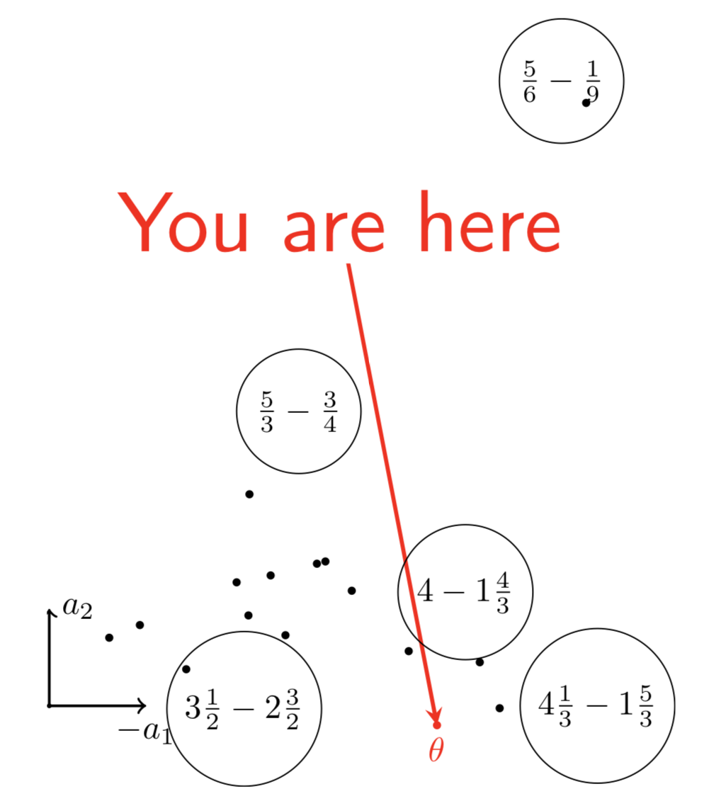 {height=8cm}
Identifier les points forts
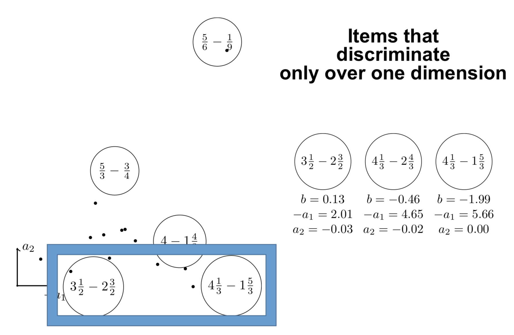 {height=8cm}
Et les points faibles
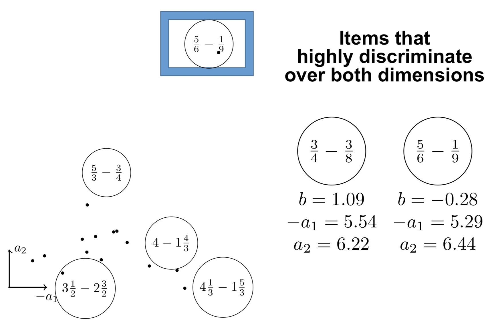 {height=8cm}
Et en grande dimension ?
\centering \includegraphics[width=0.6\linewidth]{figures/cfirt.pdf}
\raggedright \small\fullcite{Bergner2021}
Traçage de connaissances : essais d’étudiants sur exercices
Exercices de maths (ex. ASSISTments)
\centering \begin{tabular}{cccc} \toprule Items & 5 – 5 = ? & 17 – 3 = ? & 13 – 7 = ?\ \midrule New student & \alert{$\circ$} & \alert{$\circ$} & \alert{$\mathbf{\times}$}\ \bottomrule \end{tabular}
\raggedright Apprentissage d’une langue (jeu de données de Duolingo)
\includegraphics{figures/duolingo0.png}
Challenges
- Les gens peuvent faire des erreurs d’inattention
- Les connaissances évoluent au cours du temps
- Biais des données manquantes (mesurer la persévérance)
Visuellement : le traçage de connaissances (KT)
\includegraphics[width=\linewidth]{figures/dkt.png}
- Couleurs : composantes de connaissances
- Disques : résultats d’apprenants sur ces composantes
- Plein : correct
- On souhaite généraliser les connaissances à d’autres composantes
- De bleu à vert : faible à haute probabilité de répondre correctement
- Les apprenants peuvent faire plusieurs essais
Méthode
Apprendre des paramètres de questions sur des données d’historiques \hfill \emph{ex. difficulté}
Mesurer les paramètres de nouveaux apprenants \hfill \emph{ex. expertise}
De nombreux modèles pour le traçage de connaissances
\centering \includegraphics[width=\linewidth]{figures/ktm.pdf}
\includegraphics{figures/ktm-cite.pdf}
Formellement : factorization machines
Apprendre un biais \alert{$w_k$} et un embedding \alert{$\bm{v_k}$} pour chaque composante $k$ tel que : \(\logit p(\bm{x}) = \mu + \underbrace{\sum_{k = 1}^N \alert{w_k} x_k}_{\textnormal{régression logistique}} + \underbrace{\sum_{1 \leq k < l \leq N} x_k x_l \langle \alert{\bm{v_k}}, \alert{\bm{v_l}} \rangle}_{\textnormal{interactions par paires}}\)
- La théorie de la réponse à l’item multidimensionnelle en est un cas particulier.
- Permet de modéliser des informations de contexte (ex. cet exercice a été résolu sur téléphone plutôt que sur ordinateur de bureau)
\small \fullcite{rendle2012factorization}
\fullcite{Minn2018}
\fullcite{KTM2019}
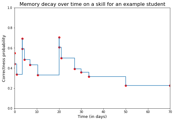
Systèmes à répétition espacée (Leitner, 1970s)
\includegraphics[width=0.5\linewidth]{figures/anki.png}\includegraphics[width=0.5\linewidth]{figures/leitner.png} \centering
Modèle de mémoire pour espacer les cartes de façon optimale
Principe simple :
- compter le nombre d’essais (heure, jour, semaine, mois, $\infty$)
- compter le nombre de succès dans ces fenêtres de temps
:::::: {.columns} ::: {.column} Apprendre par régression logistique :
- la difficulté des exercices
- la difficulté des composantes de connaissances
- le progrès par essai, par composante, par fenêtre de temps
:::
::: {.column}
 {width=100%}
:::
::::::
{width=100%}
:::
::::::
- EDM 2019
-
\scriptsize \mycite{Benoît Choffin, Fabrice Popineau, Yolaine Bourda, and Jill-Jênn Vie (2019)}{DAS3H: Modeling Student Learning and Forgetting for Optimally Scheduling Distributed Practice of Skills}{Best Paper Award at EDM 2019}
Et l’apprentissage profond dans tout ça ?
Réseaux de neurones récurrents (DKT), avec attention (SAKT, AKT)
IRT bien entraîné peut faire mieux que deep knowledge tracing (Wilson, EDM 2016).
Sur des grandes données, lorsque l’aspect séquentiel est important, des modèles profonds peuvent avoir une meilleure performance.
\fullcite{gervet2020deep}
Important de connaître les fondements, merci Michel :
\fullcite{desmarais2012review}
Europe : IA & données pour l’éducation et la formation
- Facteur humain et supervision
- Transparence
- Diversité, non discrimination et fairness (impartialité)
- Bien-être sociétal et environnemental
- Confidentialité et gouvernance des données
- Robustesse technique et sécurité
- Responsabilité
3. Diversité, non discrimination et fairness (impartialité)
- Le système est-il \alert{accessible} pour tous sans barrière ?
- Modes d’interaction appropriés pour les personnes à besoins spéciaux / interfaces appropriées
- Y a-t-il des procédures pour s’assurer que l’IA n’induira pas un traitement discriminatoire ou injuste pour ses utilisateurs ?
- La documentation du système ou son procédé d’entraînement indique-t-elle des biais potentiels dans les données ?
5. Confidentialité et gouvernance des données
- Des mécanismes sont-ils en place pour s’assurer que les données sensibles sont anonymisées et protégées pour en limiter l’accès aux personnes nécessaires ?
- Les données sont-elles traitées dans le seul but pour lequel elles ont été collectées ?
- Les enseignants ont-ils un moyen de signaler des problèmes quant à la confidentialité ou la protection des données ? En sont-ils informés ?
- Simplement : est-ce que le système respecte la RGPD ? Les paramètres de confidentialité sont-ils modifiables ?
Confidentialité
- Il est difficile d’accéder à des données sensibles (procédures très longues pour la recherche)
- Un jeu de données qui est ouvert peut être archivé pour toujours
- Pourquoi ne pas avoir plutôt accès à :
- des statistiques (cf. DEPP)
- des probabilités conditionnelles
- des modèles pré-entraînés
- des jeux de données synthétiques ? (ne serait-ce que pour la reproductibilité)
Outline
- Privacy
- Metrics: utility and re-identification
- Attack models
- Weak: Membership inference
- Strong: Train on real and fake, learn to distinguish the two
Striking facts
People pseudonymize, but it’s not enough
@narayanan2008robust managed to de-anonymize a Netflix pseudonymized dataset of seen movies with IMDb
People $k$-anonymize, but high-dimensional data (e.g. mobility) is rarely $k$-anonymizable
- 4 timestamp-location points are needed to uniquely identify 95\% of individual trajectories in a dataset of 1.5M rows \citep{de2013unique}
- 15 demographic points are enough to re-identify 99.96\% of Americans \citep{rocher2019estimating}
Differentially private graphical models
$\varepsilon$-differential privacy
\[\left|\log \frac{Pr(A(D_1) \in S)}{Pr(A(D_2) \in S)}\right| \leqslant \varepsilon\]for all datasets $D_1$ and $D_2$ that differ on a single element
for all possible subsets $S$ (of $\textnormal{Im } A$)
PrivBayes \citep{zhang2017privbayes}
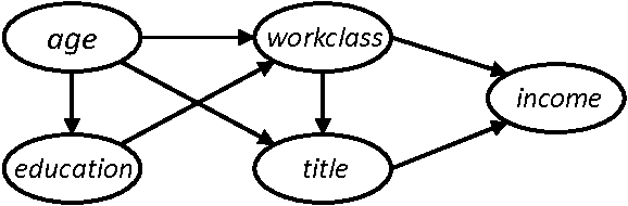 {width=50%}
However, we need a dynamic model
Intuition
Knowledge embeddings are safe to be shared
User embeddings however should be drawn from distribution
\centering
 {width=50%}
Example data
\begin{table}[h]
%\caption{Example of minimal tabular dataset.}
\label{example-dataset}
\centering
\resizebox{\textwidth}{!}{
\begin{tabular}{ccc} \toprule
user ID & action ID & outcome \ \midrule
2487 & 384 & 1
2487 & 242 & 0
2487 & 39 & 1
2487 & 65 & 1 \ \bottomrule
\end{tabular}
\arrayrulecolor{white}
\begin{tabular}{l} \toprule
description \ \midrule
user 2487 got token I'' correct \\
user 2487 got tokenate’’ incorrect
user 2487 got token an'' correct \\
user 2487 got tokenapple’’ correct \ \bottomrule
\end{tabular}
}
\arrayrulecolor{black}
\end{table}
So in our case there are two models:
- Sequence generation (Markov chain, RNN)
- Response pattern generation (IRT, Bayesian networks)
Item response theory for response pattern generation
Ex. $r_{ij}$ is 1 if user $i$ got a positive outcome on action (item) $j$
\[p_{ij} = \Pr(R_{ij} = 1) = \sigma(\theta_i + e_j)\]\noindent where $\theta_i$ is ability of user $i$ and $e_j$ is easiness of action $j$
\vspace{1cm}
Trained using Newton’s method: minimize log-loss $\mathcal{L} = \sum_{i, j} (1 - r_{ij}) \log (1 - p_{ij}) + r_{ij} \log p_{ij}$
Logistic regression with sparse features
Let us encode the event (user $i$, item $j$) as a two-hot vector $\bm{x}$:
\centering
$p_{ij} = \sigma(\langle \alert{\bm{w}}, \bm{x} \rangle) = \sigma(\sum_k \alert{w_k} x_k) = \sigma(\alert{\theta_i} + \alert{e_j})$
Utility
\centering Practictioners who conduct study on the real and fake dataset should have similar findings
$\downarrow$
Trained model on original dataset should have parameters that are not too far in RMSE
\raggedright
We also consider weighted RMSE:
\[wRMSE = \sqrt{\sum_{i = 1}^N w_i (d_i - \widehat{d_i})^2}\]where $w_i \in [0, 1]$ is the frequency of action $i$ in the training set.
Reidentification
\centering It should not be easy to re-identify people / the fake dataset should not leak too much information about participants
$\downarrow$
An attacker has to guess, from a broader population, who was in the training set
\centering \begin{tikzpicture}[ xscale=3, yscale=2, data/.style={draw}, >=stealth ] \node[data] (original) at (0,0) {Original}; \node[data] (training) at (1,0) {Training set}; \node[data] (fake) at (1,-1) {Fake set}; \node[data,text width=1.6cm,text centered] (real-irt) at (2,0) {Real item params $d$}; \node[data,text width=1.6cm,text centered] (fake-irt) at (2,-1) {Fake item params $\hat{d}$}; \draw[->] (original) edge node[above=3mm] {sampling half users} (training); \draw[->] (training) edge node[right] {generator} (fake); \draw[<->] (real-irt) edge node[right] {RMSE} (fake-irt); \draw[->,dashed,bend right] (original) edge (training); \draw[->,dashed,bend left=60,text width=2cm,text centered] (fake) edge node[below left] {reidentify\AUC} (training); \draw[->] (training) edge node[above] {IRT} (real-irt); \draw[->] (fake) edge node[above] {IRT} (fake-irt); \end{tikzpicture}
(framework inspired by NeurIPS “Hide and Seek” challenge in healthcare by \cite{jordon2020hide})
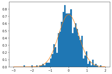
Histogram of actions ($y$-axis: frequency)
\centering
Actions
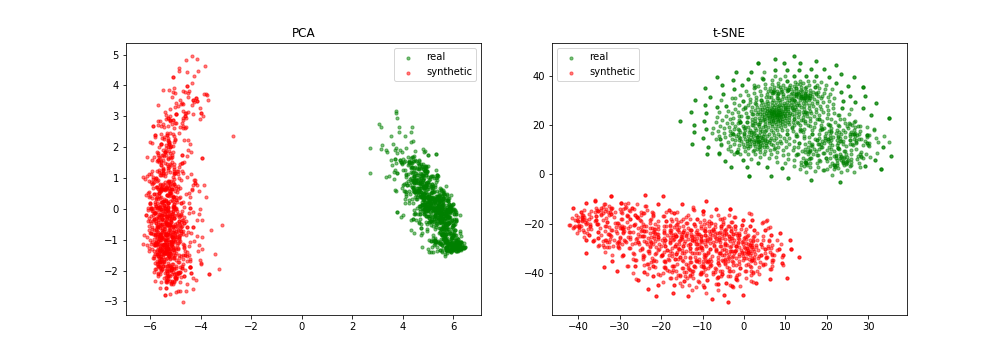
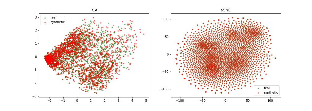
Quantitative results
{width=49%}
{width=49%}
Slided bag of events for SNDS
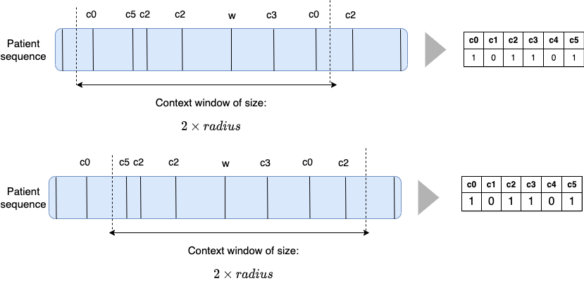
A bad example
A good example
 {width=100%}
Fairness
“Different models with the same reported accuracy can have a very different distribution of error across population” (Hardt, 2017)
\pause
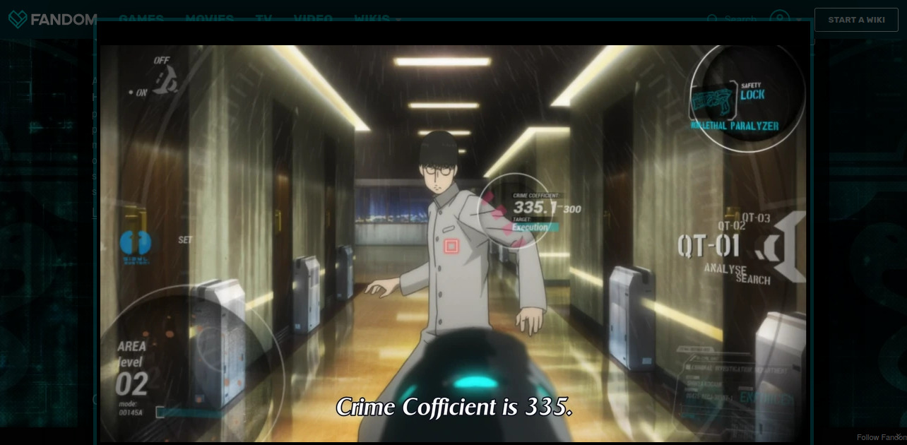
Crime prediction (watch Psycho-Pass):
Goals
- \alert{Group fairness}: positive rate in group $\simeq$ positive rate overall
- \alert{Individual fairness}: similar people receive similar outcomes
- Find a trade-off between accuracy and fairness
Useful reads
Many results are being renamed and rediscovered :(
\fullcite{hutchinson201950}
\fullcite{zemel2013learning}
Example of fairness
\centering
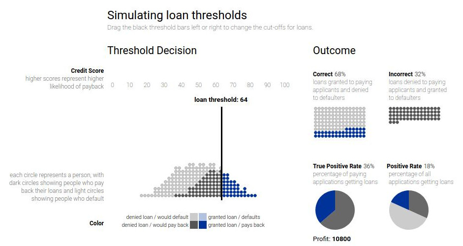 {width=100%}
See Attacking discrimination with smarter machine learning
Visually
\centering
Formally
\[M_{n, k} = P(Z = k|x_n) \propto \exp(-d(x_n, \alert{v_k}))\]\raggedleft High if $x_n$ is close to $\alert{v_k}$
\raggedright
\[\hat{x_n} = \sum_k M_{n, k} \alert{v_k}\]\only<1>{\(\displaystyle \widehat{y_n} = \sum_k M_{n, k} \alert{w_k}\)} \only<2>{\(\widehat{y_n} = \sum_k \underbrace{M_{n, k}}_{\in \{0, 1\}} \alert{w_k}\)} \only<3>{\(\widehat{y_n} = \sum_k \underbrace{M_{n, k}}_{\in \{0, 1\}} \underbrace{\alert{w_k}}_{\in \{0, 1\}}\)}
$\alert{v_k} \in \mathbf{R}^d$, $\alert{w_k} \in \mathbf{R}$ are \alert{learned}
Objective
- Accuracy
-
$L_y = \sum_n - y_n \log \hat{y_n} - (1 - y_n) \log (1 - \hat{y_n})$
- Reconstruction
-
$L_x = \sum_n x_n - \hat{x}_n ^2$ - Fairness
-
$L_z = \sum_k M_k^+ - M_k^- $
where $M_k^+ = \underbrace{\mathbb{E}+ M{n, k}}_{\textnormal{average across subgroup}}$
\only<1>{\(L = A_z L_z + A_x L_x + A_y L_y\)} \only<2>{\(L = A_z L_z + A_x L_x + A_y \alert{N_D}\)}
Baselines
LR: Logistic Regression
FNB: Fair Naive Bayes
RLR: Regularized LR
LFR: Learning Fair Representations
Results I
Accuracy (high)
Discrimination (low)
\[D = | \mathbb{E}_+ \hat{y}^n - \mathbb{E}_- \hat{y}^n |\]Results I, see paper
\centering
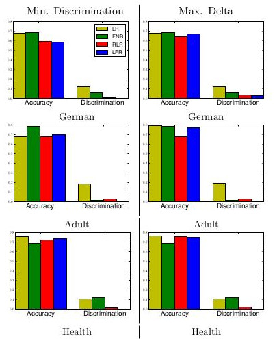 {width=70%}
Results II
Consistency (high)
\[y_{nn} = 1 - \frac1{Nk} \sum_n \left| \hat{y}_n - \sum_{j \in kNN(x_n)} \hat{y}_j \right|\]Results II
\centering
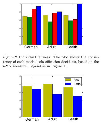 {width=60%}
Going beyond: AUC constraints
Constraints on AUC or area between ROC curves (ABROCA)
\centering
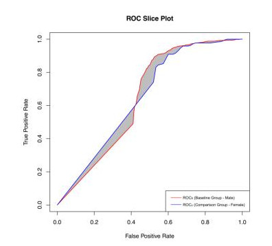 {width=60%}
\raggedright
Evaluating the Fairness of Predictive Student Models Through Slicing Analysis (Gardner, Brooks and Baker, 2019)
Also works from Bellet next door
Going beyond: Relation to differential privacy
\centering
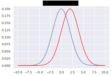 {width=60%}
\pause
\[\begin{aligned} \forall S \subset \textnormal{Im} A, \forall D_1, D_2 \textnormal{"close"}, Pr(A(D_1) \subset S) \leq e^\varepsilon Pr(A(D_2) \subset S)\\ \forall S \subset \textnormal{Im} A, \forall D_1, D_2 \textnormal{"close"} \left|\frac{\log Pr(A(D_1) \in S)}{\log Pr(A(D_2) \in S)}\right| \leq \varepsilon \end{aligned}\]\raggedright
For more on this beautiful relationship:
Fairness through Awareness (Dwork et al., 2011)
Conclusion
- Ouvrons massivement les données de gens qui n’existent pas
- Il faut mesurer les discriminations pour réduire les inégalités
\vspace{1cm}
\pause
Merci ! Questions ? \hfill Ces slides sur \href{https://jjv.ie/slides/pfia.pdf}{jjv.ie/slides/pfia.pdf}