% Optimizing Human Learning % Fabrice Popineau \and \alert{Jill-Jênn Vie} \and Michal Valko\newline RIKEN AIP\newline\newline\includegraphics[height=1.2cm]{figures/cs.png}\qquad\includegraphics[height=1cm]{figures/aip-logo.png}\qquad\includegraphics[height=1.3cm]{figures/inria.jpg} % August 21, 2019 — theme: Frankfurt section-titles: false handout: true biblio-style: authoryear header-includes: - \usepackage{booktabs} - \usepackage{multicol} - \usepackage{bm} - \usepackage{multirow} - \DeclareMathOperator\logit{logit} - \def\ReLU{\textnormal{ReLU}} - \newcommand\mycite[3]{\textcolor{blue}{#1} “#2”.~#3.} biblatexoptions: - maxbibnames=99 - maxcitenames=5 —

Introduction

Optimizing Human Learning

We observe data collected by a platform (ITS, MOOC, etc.)

We can learn a \alert{generative model of the world} ($\sim$ knowledge tracing)
Then learn a policy to optimize it (e.g. this workshop)

Challenges

• Representations that evolve over time
  (actions from the teacher can modify the learner)
• \alert{Which objective function should be optimized?}
• New users \& items appear (cold-start)
• Sequential learning requires a measure of uncertainty
• High-stakes applications require interpretability

Choosing the objective function to optimize

\alert{Maximize information} $\rightarrow$ learners fail 50% of the time (good for the assessing institution, not for the learning student)

\alert{Maximize success rate} $\rightarrow$ asking too easy questions

\alert{Maximize the growth of the success rate} (Clement et al. 2015)

\alert{Compromise exploration} (items that we don’t know)
and \alert{exploitation} (items that measure well)

\alert{Identify a gap from the learner} (Teng et al. ICDM 2018)

• assume that a item brings less learning when it was administered before (Seznec et al. AISTATS 2019, SequeL)

Increasing number of works(hops) about reinforcement learning in education

Predicting student performance

Data

A population of students answering questions

• Events: “Student $i$ answered question $j$ correctly/incorrectly”

Goal

• Learn the difficulty of questions automatically from data
• Measure the knowledge of students
• Potentially optimize their learning

Assumption

Good model for prediction $\rightarrow$ Good adaptive policy for teaching

Learning outcomes of this tutorial

• \alert{Logistic regression} is amazing
  • Unidimensional
  • Takes IRT, PFA as special cases\vspace{1cm}
• \alert{Factorization machines} are even more amazing
  • Multidimensional
  • Take MIRT as special case\vspace{1cm}
• It makes sense to consider \alert{deep neural networks}
  • What does deep knowledge tracing model exactly?

Families of models

• Factorization Machines [@rendle2012factorization]
  • Multidimensional Item Response Theory
  • Logistic Regression
    • Item Response Theory
    • Performance Factor Analysis
• Recurrent Neural Networks
  • Deep Knowledge Tracing [@piech2015deep]

\vspace{5mm}

\fullcite{rendle2012factorization}

\fullcite{piech2015deep}

Problems

Weak generalization

Filling the blanks: some students did not attempt all questions

Strong generalization

Cold-start: some new students are not in the train set

Dummy dataset

\begin{columns} \begin{column}{0.6\linewidth} \begin{itemize} \item User 1 answered Item 1 correct \item User 1 answered Item 2 incorrect \item User 2 answered Item 1 incorrect \item User 2 answered Item 1 correct \item User 2 answered Item 2 ??? \end{itemize} \end{column} \begin{column}{0.4\linewidth} \centering \input{tables/dummy-ui}\vspace{5mm}

\texttt{dummy.csv} \end{column} \end{columns}

Logistic Regression

Task 1: Item Response Theory

Learn abilities $\theta_i$ for each user $i$
Learn easiness $e_j$ for each item $j$ such that: \(\begin{aligned} Pr(\textnormal{User $i$ Item $j$ OK}) & = \sigma(\theta_i + e_j)\\ \logit Pr(\textnormal{User $i$ Item $j$ OK}) & = \theta_i + e_j \end{aligned}\)

Logistic regression

Learn $\alert{\bm{w}}$ such that $\logit Pr(\bm{x}) = \langle \alert{\bm{w}}, \bm{x} \rangle$

Usually with L2 regularization: ${

\bm{w}

}_2^2$ penalty $\leftrightarrow$ Gaussian prior

Graphically: IRT as logistic regression

Encoding of “User $i$ answered Item $j$”:

\centering

\[\logit Pr(\textnormal{User $i$ Item $j$ OK}) = \langle \bm{w}, \bm{x} \rangle = \theta_i + e_j\]

Encoding

python encode.py --users --items

\centering

\input{tables/show-ui}

data/dummy/X-ui.npz

\raggedright Then logistic regression can be run on the sparse features:

python lr.py data/dummy/X-ui.npz

Oh, there’s a problem

python encode.py --users --items

python lr.py data/dummy/X-ui.npz

\input{tables/pred-ui}

We predict the same thing when there are several attempts.

Count successes and failures

Keep track of what the student has done before:

\centering

\input{tables/dummy-uiswf}

data/dummy/data.csv

Task 2: Performance Factor Analysis

$W_{ik}$: how many successes of user $i$ over skill $k$ ($F_{ik}$: #failures)

Learn $\alert{\beta_k}$, $\alert{\gamma_k}$, $\alert{\delta_k}$ for each skill $k$ such that: \(\logit Pr(\textnormal{User $i$ Item $j$ OK}) = \sum_{\textnormal{Skill } k \textnormal{ of Item } j} \alert{\beta_k} + W_{ik} \alert{\gamma_k} + F_{ik} \alert{\delta_k}\)

python encode.py --skills --wins --fails

\centering \input{tables/show-swf}

data/dummy/X-swf.npz

Better!

python encode.py --skills --wins --fails

python lr.py data/dummy/X-swf.npz

\input{tables/pred-swf}

Task 3: a new model (but still logistic regression)

python encode.py --items --skills --wins --fails

python lr.py data/dummy/X-iswf.npz

Factorization Machines

Here comes a new challenger

How to model \alert{side information} in, say, recommender systems?

Logistic Regression

Learn a \alert{bias} for each feature (each user, item, etc.)

Factorization Machines

Learn a \alert{bias} and an \alert{embedding} for each feature

What can be done with embeddings?

\centering

{width=60%}

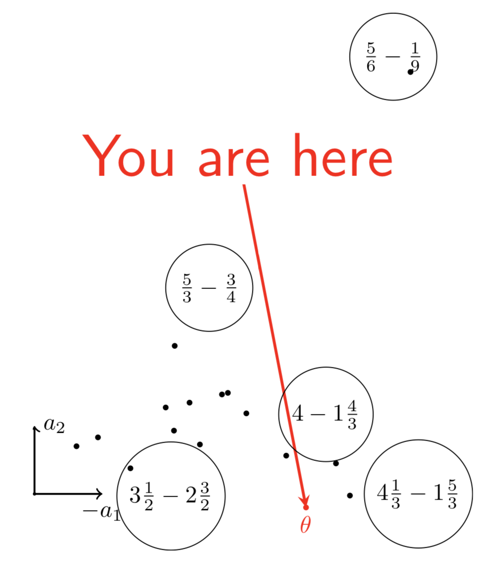
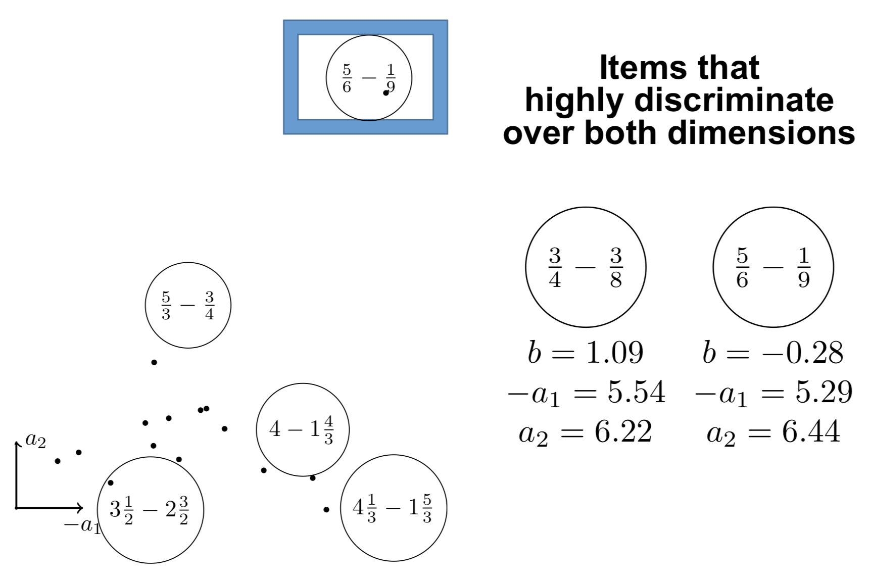
Interpreting the components

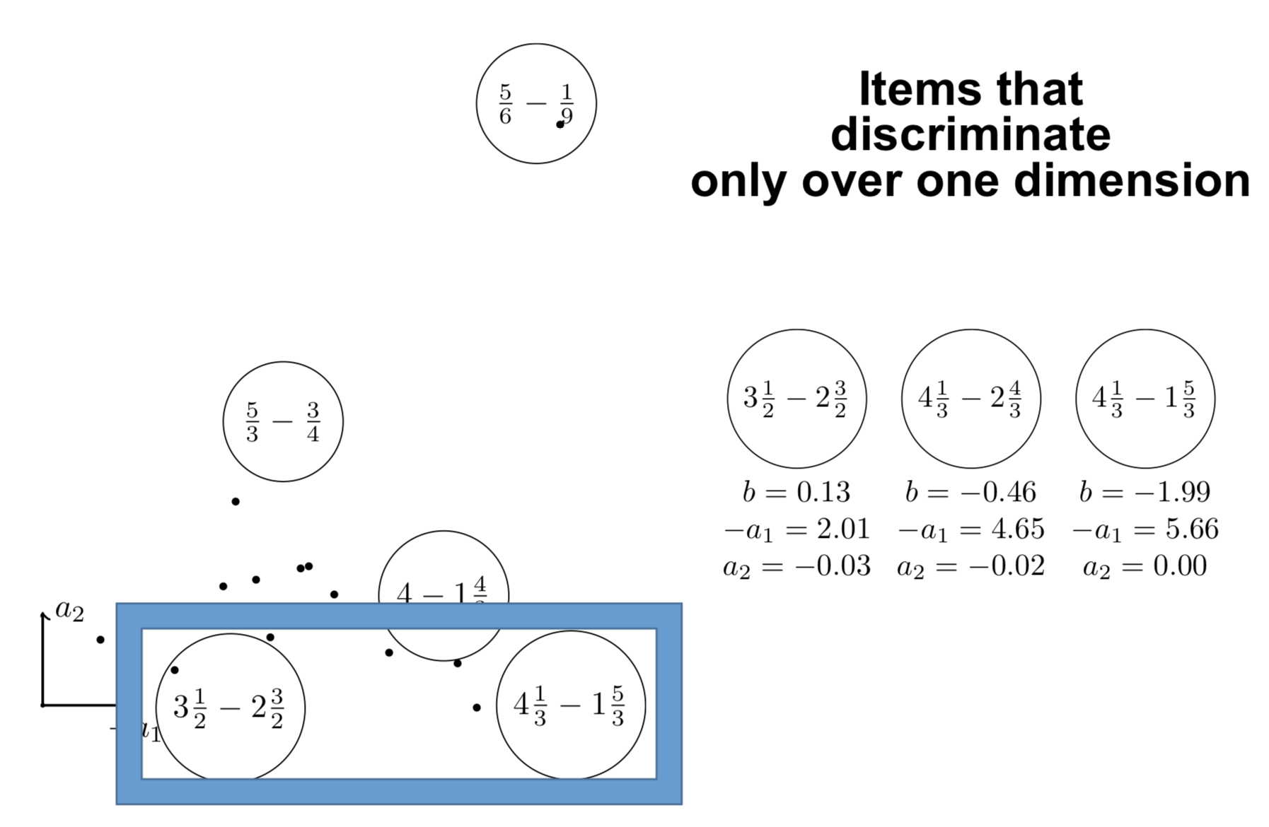
Interpreting the components

Graphically: logistic regression

\centering

How to model pairwise interactions with side information?

If you know user $i$ attempted item $j$ on \alert{mobile} (not desktop)
How to model it?

$y$: score of event “user $i$ solves correctly item $j$”

IRT

\[y = \theta_i + e_j\]

Multidimensional IRT (similar to collaborative filtering)

\[y = \theta_i + e_j + \langle \bm{v_{\textnormal{user $i$}}}, \bm{v_{\textnormal{item $j$}}} \rangle\]

\pause

With side information

\small \vspace{-3mm} \(y = \theta_i + e_j + \alert{w_{\textnormal{mobile}}} + \langle \bm{v_{\textnormal{user $i$}}}, \bm{v_{\textnormal{item $j$}}} \rangle + \langle \bm{v_{\textnormal{user $i$}}}, \alert{\bm{v_{\textnormal{mobile}}}} \rangle + \langle \bm{v_{\textnormal{item $j$}}}, \alert{\bm{v_{\textnormal{mobile}}}} \rangle\)

Graphically: factorization machines

\centering

Formally: factorization machines

Learn bias \alert{$w_k$} and embedding \alert{$\bm{v_k}$} for each feature $k$ such that: \(\logit p(\bm{x}) = \mu + \underbrace{\sum_{k = 1}^N \alert{w_k} x_k}_{\textnormal{logistic regression}} + \underbrace{\sum_{1 \leq k < l \leq N} x_k x_l \langle \alert{\bm{v_k}}, \alert{\bm{v_l}} \rangle}_{\textnormal{pairwise interactions}}\)

\begin{block}{Particular cases} \begin{itemize} \item Multidimensional item response theory: $\logit p = \langle \bm{u_i}, \bm{v_j} \rangle + e_j$ \item SPARFA: $\bm{v_j} > \bm{0}$ and $\bm{v_j}$ sparse \item GenMA: $\bm{v_j}$ is constrained by the zeroes of a q-matrix $(q_{ij})_{i, j}$ \end{itemize} \end{block}

\footnotesize \fullcite{lan2014sparse}

\fullcite{Vie2016ECTEL}

Assistments 2009 dataset

278608 attempts of 4163 students over 196457 items on 124 skills.

• Download http://jiji.cat/weasel2018/data.csv
• Put it in data/assistments09

python fm.py data/assistments09/X-ui.npz
etc. or make big

\vspace{1cm}

\input{tables/results}

Results obtained with FM $d = 20$

Benchmarks

\centering \footnotesize \begin{tabular}{cccc} \toprule Model & Component & Size & AUC\ \midrule Bayesian Knowledge Tracing & Hidden Markov Model & \multirow{2}{}{$2N$} & \multirow{2}{}{0.63}
(Corbett and Anderson 1994) & \ \midrule Deep Knowledge Tracing & Recurrent Neural Network & \multirow{2}{}{$O(Nd + d^2)$} & \multirow{2}{}{0.75}
(Piech et al. 2015) & \ \midrule \only<2->{Item Response Theory & Logistic Regression & \multirow{3}{}{$N$} & \multirow{3}{}{0.76}\} \only<2->{(Rasch 1960) & online\} \only<2->{(Wilson et al. 2016) \ \midrule} \only<2->{Knowledge Tracing Machines & Factorization Machines & $Nd + N$ & \alert{0.82}\ \bottomrule} \end{tabular}

AAAI 2019

\scriptsize\mycite{Jill-Jênn Vie and Hisashi Kashima (2019)}{Knowledge Tracing Machines: Factorization Machines for Knowledge Tracing}{Proceedings of the 33th AAAI Conference on Artificial Intelligence}

Impact on learning: modeling forgetting

Optimize scheduling of items in spaced repetition systems ($\sim$ Anki)

\centering \includegraphics[width=0.5\linewidth]{figures/anki.png}

\raggedright Use knowledge tracing machines with extra features: counters of attempts at skill level for different time windows in the past

EDM 2019

\scriptsize \mycite{Benoît Choffin, Fabrice Popineau, Yolaine Bourda, and Jill-Jênn Vie (2019)}{DAS3H: Modeling Student Learning and Forgetting for Optimally Scheduling Distributed Practice of Skills}{\alert{Best Paper Award}}

Deep Learning

Deep Factorization Machines

Learn layers \alert{$W^{(\ell)}$} and \alert{$b^{(\ell)}$} such that: \(\begin{aligned}[c] \bm{a}^{0}(\bm{x}) & = (\alert{\bm{v_{\texttt{user}}}}, \alert{\bm{v_{\texttt{item}}}}, \alert{\bm{v_{\texttt{skill}}}}, \ldots)\\ \bm{a}^{(\ell + 1)}(\bm{x}) & = \ReLU(\alert{W^{(\ell)}} \bm{a}^{(\ell)}(\bm{x}) + \alert{\bm{b}^{(\ell)}}) \quad \ell = 0, \ldots, L - 1\\ y_{DNN}(\bm{x}) & = \ReLU(\alert{W^{(L)}} \bm{a}^{(L)}(\bm{x}) + \alert{\bm{b}^{(L)}}) \end{aligned}\)

\[\logit p(\bm{x}) = y_{FM}(\bm{x}) + y_{DNN}(\bm{x})\]

\fullcite{Duolingo2018}

Comparison

• FM: $y_{FM}$ factorization machine with $\lambda = 0.01$
• Deep: $y_{DNN}$: multilayer perceptron
• DeepFM: $y_{DNN} + y_{FM}$ with shared embedding
• Bayesian FM: $\alert{w_k}, \alert{v_{kf}} \sim \mathcal{N}(\alert{\mu_f}, 1/\alert{\lambda_f})$
  $\alert{\mu_f} \sim \mathcal{N}(0, 1)$, $\alert{\lambda_f} \sim \Gamma(1, 1)$ (trained using Gibbs sampling)

Various types of side information

• first: <discrete> (user, token, countries, etc.)
• last: <discrete> + <continuous> (time + days)
• pfa: <discrete> + wins + fails

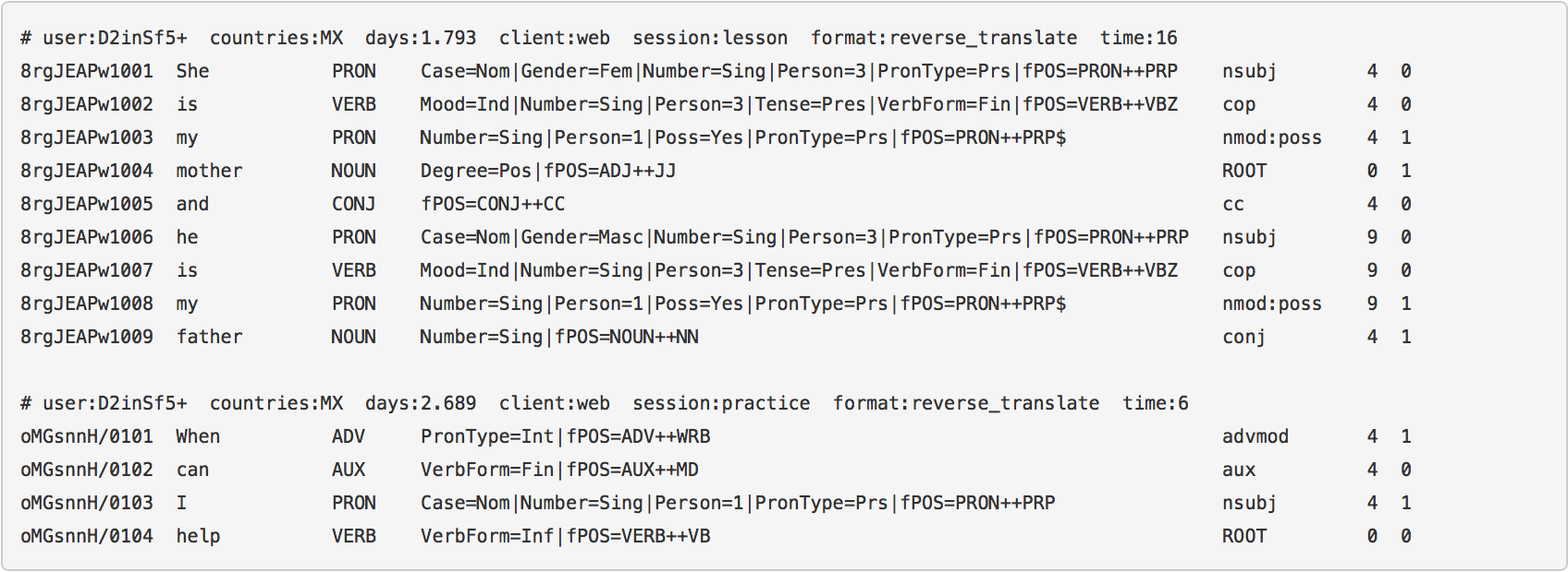
Duolingo dataset

Results

\begin{tabular}{cccccccc} \toprule Model & $d$ & epoch & train & first & last & pfa
\midrule Bayesian FM & 20 & 500/500 & – & 0.822 & – & –
Bayesian FM & 20 & 500/500 & – & – & 0.817 & –
DeepFM & 20 & 15/1000 & 0.872 & 0.814 & – & –
Bayesian FM & 20 & 100/100 & – & – & 0.813 & –
FM & 20 & 20/1000 & 0.874 & 0.811 & – & –
Bayesian FM & 20 & 500/500 & – & – & – & 0.806
FM & 20 & 21/1000 & 0.884 & – & – & 0.805
FM & 20 & 37/1000 & 0.885 & – & 0.8 & –
DeepFM & 20 & 77/1000 & 0.89 & – & 0.792 & –
Deep & 20 & 7/1000 & 0.826 & 0.791 & – & –
Deep & 20 & 321/1000 & 0.826 & – & 0.79 & –
LR & 0 & 50/50 & – & – & – & 0.789
LR & 0 & 50/50 & – & 0.783 & – & –
LR & 0 & 50/50 & – & – & 0.783 & –
\bottomrule \end{tabular}

Duolingo ranking

\centering

\begin{tabular}{cccc} \toprule Rank & Team & Algo & AUC\ \midrule 1 & SanaLabs & RNN + GBDT & .857
2 & singsound & RNN & .854
2 & NYU & GBDT & .854
4 & CECL & LR + L1 (13M feat.) & .843
5 & TMU & RNN & .839\ \midrule 7 (off) & JJV & Bayesian FM & .822
8 (off) & JJV & DeepFM & .814
10 & JJV & DeepFM & .809\ \midrule 15 & Duolingo & LR & .771\ \bottomrule \end{tabular}

\raggedright \small \fullcite{Settles2018}

What ‘bout recurrent neural networks?

Deep Knowledge Tracing: model the problem as sequence prediction

• Each student on skill $q_t$ has performance $a_t$
• How to predict outcomes $\bm{y}$ on every skill $k$?
• Spoiler: by measuring the evolution of a latent state $\alert{\bm{h_t}}$

\small \fullcite{piech2015deep} \normalsize

Our approach: encoder-decoder

\def\xin{\bm{x^{in}_t}} \def\xout{\bm{x^{out}_t}} \(\left\{\begin{array}{ll} \bm{h_t} = Encoder(\bm{h_{t - 1}}, \xin)\\ p_t = Decoder(\bm{h_t}, \xout)\\ \end{array}\right. t = 1, \ldots, T\)

Graphically: deep knowledge tracing

\centering

Deep knowledge tracing with dynamic student classification

\centering

\normalsize

ICDM 2018

\scriptsize\mycite{Sein Minn, Yi Yu, Michel Desmarais, Feida Zhu, and Jill-Jênn Vie (2018)}{Deep Knowledge Tracing and Dynamic Student Classification for Knowledge Tracing}{Proceedings of the 18th IEEE International Conference on Data Mining}

DKT seen as encoder-decoder

\centering

Results on Fraction dataset

500 middle-school students, 20 Fraction subtraction questions,
8 skills (full matrix)

\begin{table} \centering \begin{tabular}{cccccc} \toprule Model & Encoder & Decoder & $\xout$ & ACC & AUC\ \midrule \textbf{Ours} & GRU $d = 2$ & bias & iswf & \textbf{0.880} & \textbf{0.944}
KTM & counter & bias & iswf & 0.853 & 0.918
PFA & counter & bias & swf & 0.854 & 0.917
Ours & $\varnothing$ & bias & iswf & 0.849 & 0.917
Ours & GRU $d = 50$ & $\varnothing$ & & 0.814 & 0.880
DKT & GRU $d = 2$ & $d = 2$ & s & 0.772 & 0.844
Ours & GRU $d = 2$ & $\varnothing$ & & 0.751 & 0.800\ \bottomrule \end{tabular} \label{results-fraction} \end{table}

Results on Berkeley dataset

562201 attempts of 1730 students over 234 CS-related items of 29 categories.

\begin{table} \centering \begin{tabular}{cccccc} \toprule Model & Encoder & Decoder & $\xout$ & ACC & AUC\ \midrule \textbf{Ours} & GRU $d = 50$ & bias & iswf & \textbf{0.707} & \textbf{0.778}
\textbf{KTM} & counter & bias & iswf & \textbf{0.704} & \textbf{0.775}
Ours & $\varnothing$ & bias & iswf & 0.700 & 0.770
DKT & GRU $d = 50$ & $d = 50$ & s & 0.684 & 0.751
Ours & GRU $d = 100$ & $\varnothing$ & & 0.682 & 0.750
PFA & counter & bias & swf & 0.630 & 0.683
DKT & GRU $d = 2$ & $d = 2$ & s & 0.637 & 0.656\ \bottomrule \end{tabular} \label{results-assistments} \end{table}

\raggedright \small \fullcite{Vie2019encode}

Conclusion

Take home message

\alert{Factorization machines} are a strong baseline for knowledge tracing that take many models as special cases

\alert{Recurrent neural networks} are powerful because they track the evolution of the latent state (try simpler dynamic models?)

\alert{Deep factorization machines} may require more data/tuning, but neural collaborative filtering offer promising directions

Next step: use this model and optimize human learning

Any suggestions are welcome!

Feel free to chat:

\centering vie@jill-jenn.net

\raggedright All code:

\centering github.com/jilljenn/ktm

\raggedright Do you have any questions?