Jill-Jênn Vie

Researcher at Inria

% Modeling uncertainty for policy learning in education % Jill-Jênn Vie¹; Tomas Rigaux¹; Koh Takeuchi²; Hisashi Kashima² % ¹ Inria Saclay, SODA team\newline ² Kyoto University — aspectratio: 169 handout: false institute: \hfill \includegraphics[height=1cm]{figures/inria.png} \includegraphics[height=1cm]{figures/kyoto.png} section-titles: false theme: metropolis header-includes: - \usepackage{bm} - \usepackage{multicol,booktabs} - \usepackage{algorithm,algpseudocode,algorithmicx} - \DeclareMathOperator\argmax{argmax} - \DeclareMathOperator\logit{logit} - \def\bm{\boldsymbol} - \def\u{\bm{u}} - \def\v{\bm} - \def\X{\bm{X}} - \def\x{\bm{x}} - \def\y{\bm{y}} - \def\E{\mathbb{E}} - \def\F{\mathcal{F}} - \def\I{\mathcal{I}} - \def\N{\mathcal{N}} - \def\Lb{\mathcal{L}_B} - \def\KL{\textnormal{KL}} - \metroset{sectionpage=none} —

About me

Hi, I’m JJ \hfill \only<2-3>{Jill = \includegraphics{jill} $\neq$ Giroud}

Positive prompts: \includegraphics{anime} \hfill Negative prompts: world cup, world history

\centering \pause \pause

{width=50%}

Policy learning

Psychometrics (50s-60s): measuring \alert{latent constructs $\theta$} of examinees
given their \alert{observed answers $X$} to a questionnaire
Led to computerized adaptive tests (70s)

\centering

:::::: {.columns} ::: {.column} \raggedleft ::: ::: {.column} {width=60%} ::: ::::::

Learner $p(X \theta)$
Teacher $\pi(j X)$ based on estimate $q(\theta X)$

$X = {(\underbrace{j_t}{\in {1, \ldots, M}}, \underbrace{r{ij_t}}_{\in {0, 1}})}_t$

Example for $\theta \in \mathbb{R}$

\centering

Example for $\theta \in \mathbb{R}^2$: prior

\centering

Example for $\theta \in \mathbb{R}^2$: prior and posterior

\centering

Cross-validation of policies

\centering

Green: interactive training set \hfill Red: validation set

Goals

Previous work

PhD: assume $\theta$ does not evolve over time and learn good $\pi$
Applied it to Pix.fr French certification of digital competencies
(now in the French Code of Education; passed by 6M active users)
Pix is free software: https://github.com/1024pix/pix
Postdoc: assume $\theta$ can evolve and build better model $p(X \theta)$

Ongoing work

If data $X$ was collected by $\pi$ how to evaluate $\pi’$?
Measuring the treatment effect whether question $j$ was asked or not

Graphical models for knowledge tracing

\centering

{width=90%}

:::::: {.columns} ::: {.column width=”15%”} ::: ::: {.column width=”15%”} ::: ::: {.column width=”70%”} $p(x_{1:N}, z_{1:N}) = p(z_1) \prod_{n = 2}^N p(z_n|z_{n - 1}) \prod_{n = 1}^N p(x_n|z_n)$

$p(V) = \prod_{v \in V} p(v|\textnormal{parents}(v))$ ::: ::::::

Graphical models for knowledge tracing

\centering

{width=90%}

\raggedright

Modeling learning using HMM

or LSTM: $\hat\theta = f_\psi(X_{1:t}) = f_\psi\left(\left{(j_t, r_{ij_t})\right}_t\right)$
i.e. deep knowledge tracing (Piech et al., NeurIPS 2015)

Rewards

Pure exploitation (of information) if no prior

We want to maximize (log) likelihood: $\argmax_\theta \log p(X|\theta)$ or $\E_{p(\theta)} LL(X|\theta)$
i.e. find its zeroes or go in the direction of gradient $\nabla_\theta LL$

Property: $\E_{p(X

\theta)} \nabla_\theta LL = 0$ at the true $\theta$ parameter

If $Var_{p(X

\theta)}(\nabla_\theta LL)$ is low, the observation brings few information

\[\I(\theta) = Var_{p(X|\theta)} (\nabla_\theta LL) = -E_{p(X|\theta)} \nabla^2_\theta LL\]

Interesting because (Cramér-Rao bound): $Var(\hat\theta) \geq \I(\theta)^{-1}$

Another index for choosing a question (Chang and Ying, 1996):

\[KLI(\theta) = \int_{B(\theta, r_n)} KL_{X}(\theta_0||\theta) d\theta_0 = \int_{B(\theta, r_n)} \E_{p(X|\theta_0)} \log \frac{p(X|\theta_0)}{p(X|\theta)} \quad r_n \to 0\]

Pure exploitation: a toy example

Taking the simple model $p_j \triangleq p(X_j=1

\theta) = \sigma(\theta - d_j)$

$\nabla_\theta LL = X_j - p_j$

$\I(\theta) = -\E_{p(X

\theta)} \nabla^2_\theta LL = p_j (1 - p_j)$

So in the scalar case, the item of maximum Fisher information is the one of probability \alert{closest to 1/2}, given the current maximum likelihood estimate.

Rewards

\alert{Maximize information} $\to$ learners fail 50% of the time (good for the examiner, not for the learners)

\alert{Minimize uncertainty} i.e. the entropy of $p(\theta

X)$

\alert{Maximize success rate} $\to$ we ask too easy questions

\alert{Maximize the growth of success rate} $\to$ Clement et al. (JEDM 2015) they use $\varepsilon$-greedy where the reward is: success rate over $k$ latest attempts minus success rate over the $k$ previous attempts.

What we are interested in: measuring precisely the knowledge of student without making them fail too much.

Introduction

Outline

Preference elicitation

Getting new info from new users is hard
We need \alert{side information} and to \alert{model uncertainty}

Factorization Machines (FMs)

FMs are a generalization of latent factor models (Rendle, 2012)
Used for both regression and classification
Sometimes better than their deep counterparts

In this paper

Variational Factorization Machines
Variational: Bayesian inference $\to$ optimization

Recommender Systems

Recommender Systems as Matrix Completion

Problem

Every user rates few items (1 %)
How to infer missing ratings?

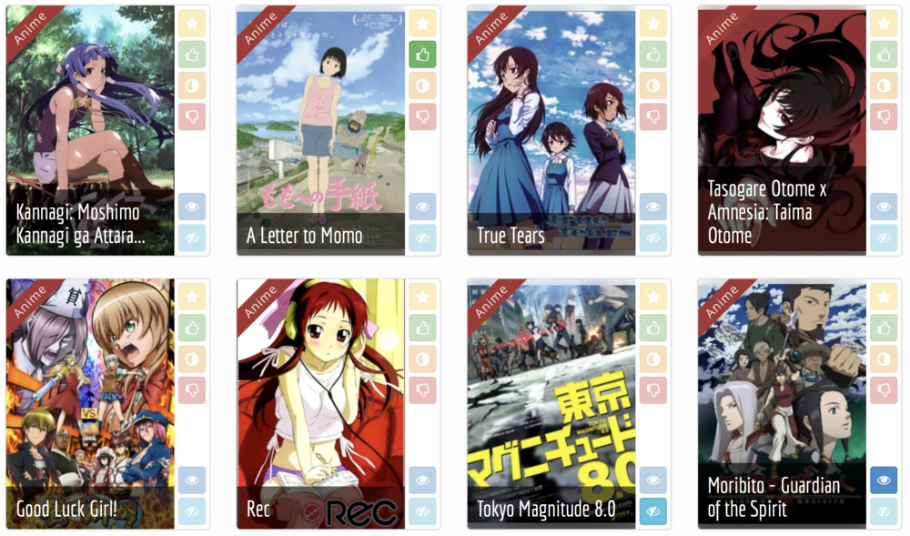
Example

\centering \begin{tabular}{ccccc} & \includegraphics[height=2.5cm]{figures/1.jpg} & \includegraphics[height=2.5cm]{figures/2.jpg} & \includegraphics[height=2.5cm]{figures/3.jpg} & \includegraphics[height=2.5cm]{figures/4.jpg}
Satoshi & ? & 5 & 2 & ?
Kasumi & 4 & 1 & ? & 5
Takeshi & 3 & 3 & 1 & 4
Joy & 5 & ? & 2 & ? \end{tabular}

Recommender Systems as Matrix Completion

Problem

Every user rates few items (1 %)
How to infer missing ratings?

Example

\centering \begin{tabular}{ccccc} & \includegraphics[height=2.5cm]{figures/1.jpg} & \includegraphics[height=2.5cm]{figures/2.jpg} & \includegraphics[height=2.5cm]{figures/3.jpg} & \includegraphics[height=2.5cm]{figures/4.jpg}
Satoshi & \alert{3} & 5 & 2 & \alert{2}
Kasumi & 4 & 1 & \alert{4} & 5
Takeshi & 3 & 3 & 1 & 4
Joy & 5 & \alert{2} & 2 & \alert{5} \end{tabular}

Preference Elicitation: select an informative batch of $K$ items

\centering

{width=90%}

Preference Elicitation: learn user embeddings in latent space

\centering

\includegraphics{figures/svd2.png}

Matrix factorization for collaborative filtering

Approximate $R$ ratings $n \times m$ by learning embeddings for user and item

\[\left.\begin{array}{r} U \textnormal{ user embeddings } n \times d\\ V \textnormal{ item embeddings } m \times d \end{array}\right\} \textnormal{ such that } R \simeq \alert{UV^T}\]

\begin{block}{Fit} Learn $U$ and $V$ to \alert{minimize} $ {||R - UV^T||}_2^2 + \lambda \cdot \textnormal{regularization} $ \end{block}

\begin{block}{Predict: Will user $i$ like item $j$?} Just compute $\langle \u_i, \v_j \rangle$ \end{block}

The actual model also contains bias terms for user $i$ and item $j$

\[r_{ij} = \mu + \alert{w^u_i + w^v_j} + \langle \u_i, \v_j \rangle\]

How to model side information?

If you know user $i$ watched item $j$ at the \alert{cinema} (or on TV, or on smartphone), how to model it?

$r_{ij}$: rating of user $i$ on item $j$

Collaborative filtering

\[r_{ij} = w_{\textnormal{user } i} + w_{\textnormal{item } j} + \langle \bm{v}_{\textnormal{user $i$}}, \bm{v}_{\textnormal{item $j$}} \rangle\]

\pause

With side information

\[r_{ij} = w_{\textnormal{user } i} + w_{\textnormal{item } j} + \alert{w_{cinema}} + \langle \bm{v}_{\textnormal{user $i$}}, \bm{v}_{\textnormal{item $j$}} \rangle + \langle \bm{v}_{\textnormal{user $i$}}, \alert{\bm{v}_{\textnormal{cinema}}} \rangle + \langle \bm{v}_{\textnormal{item $j$}}, \alert{\bm{v}_{\textnormal{cinema}}} \rangle\]

Encoding the problem using sparse features

\centering \begin{tabular}{rrr|rrrr|rrr} \toprule \multicolumn{3}{c}{Users} & \multicolumn{4}{c}{Items} & \multicolumn{3}{c}{Formats}
\cmidrule{1-3} \cmidrule{4-6} \cmidrule{7-10} $U_1$ & $U_2$ & $U_3$ & $I_1$ & $I_2$ & $I_3$ & $I_4$ & cinema & TV & mobile
\midrule 0 & \alert1 & 0 & 0 & \alert1 & 0 & 0 & 0 & \alert1 & 0
0 & 0 & \alert1 & 0 & 0 & \alert1 & 0 & 0 & \alert1 & 0
0 & \alert1 & 0 & 0 & 0 & \alert1 & 0 & \alert1 & 0 & 0
0 & \alert1 & 0 & 0 & \alert1 & 0 & 0 & \alert1 & 0 & 0
\alert1 & 0 & 0 & 0 & 0 & 0 & \alert1 & 0 & \alert1 & 0
\bottomrule \end{tabular}

Graphically: factorization machines

\centering

Formally: factorization machines

Learn bias \alert{$w_k$} and embedding \alert{$\bm{v_k}$} for each feature $k$ such that: $y(\bm{x}) = \mu + \underbrace{\sum_{k = 1}^K \alert{w_k} x_k}_{\textnormal{linear regression}} + \underbrace{\sum_{1 \leq k < l \leq K} x_k x_l \langle \alert{\bm{v_k}}, \alert{\bm{v_l}} \rangle}_{\textnormal{pairwise interactions}}$

This model is for regression
If classification, use a link function like softmax/sigmoid or Gaussian CDF

\small \fullcite{rendle2012factorization}

Training using, for example, SGD

Take a batch $(\X_B, y_B)$ and update the parameters such that the error is minimized.

Loss in classification: cross-entropy
Loss in regression: squared error

\begin{algorithm}[H] \begin{algorithmic} \For {batch $\bm{X}_B, y_B$} \For {$k$ feature involved in this batch $\bm{X}_B$} \State Update $w_k, \bm{v}_k$ to decrease loss estimate $\mathcal{L}$ on $\bm{X}_B$ \EndFor \EndFor \end{algorithmic} \caption{SGD} \label{algo-vfm} \end{algorithm}

Bayesian variational inference

Why do we prefer distributions over point estimates?

Because we can measure \alert{uncertainty}
More robust for critical applications
Can guide sequential estimation (preference elicitation)

Variational inference

\only<1>{Approximate true posterior with an easier distribution (Gaussian)}

\only<2>{\begin{align} \textnormal{Priors } p(w_k) = \N(\nu^w_{g(k)}, 1/\lambda^w_{g(k)}) \qquad p(v_{kf}) = \N(\nu^{v,f}_{g(k)}, 1/\lambda^{v,f}_{g(k)})
\textnormal{Approx. posteriors } q(w_k) = \N(\mu^w_k, (\sigma^w_k)^2) \qquad q(v_{kf}) = \N(\mu^{v,f}_k, (\sigma^{v,f}_k)^2) \end{align}}

Idea: increase the ELBO $\Rightarrow$ increase the objective

\begin{align} \log p(\y) & \geq \sum_{i = 1}^N \underbrace{\E_{q(\theta)} [\log p(y_i|x_i,\theta)] - \KL(q(\theta)||p(\theta))}_{\textrm{Evidence Lower Bound (ELBO) }}
& \quad = \sum_{i = 1}^N \E_{q(\theta)} [ \log p(y_i|x_i,\theta) ] - \KL(q(w_0)||p(w_0)) - \sum_{k = 1}^K \KL(q(\theta_k)||p(\theta_k)) \end{align}

Needs to be rescaled for mini-batching (see in the paper)

Graphically: Variational Factorization Machines

\centering

VFM training

\begin{algorithm}[H] \begin{algorithmic} \For {each batch $B \subseteq {1, \ldots, N}$} \State Sample $w_0 \sim q(w_0)$ \For {$k \in F(B)$ feature involved in batch $B$} \State Sample $S$ times $w_k \sim q(w_k)$, $\bm{v}_k \sim q(\bm{v}_k)$ \EndFor \For {$k \in F(B)$ feature involved in batch $B$} \State Update parameters $\mu_k^w, \sigma_k^w, \bm{\mu}_k^v, \bm{\sigma}_k^v$ to increase ELBO estimate \EndFor \State Update hyper-parameters $\mu_0, \sigma_0, \nu, \lambda, \alpha$ \State Keep a moving average of the parameters to compute mean predictions \EndFor \end{algorithmic} \caption{Variational Training (SGVB) of FMs} \label{algo-vfm} \end{algorithm} \vspace{-5mm} Then $\sigma$ can be reused for preference elicitation (see how in the paper)

Stochastic weight averaging

A beneficial regularization: keep all weights over training epochs and average them.

Connections to Polyak-Ruppert averaging, aka stochastic weight averaging

Experiments on real data

\centering \begin{tabular}{llrrrr} \toprule Task & Dataset & #users & #items & #entries & Sparsity
\midrule %fraction & 536 & 20 & 10720 & 0.000
%duolingo & 1213 & 2417 & 1064228 & 0.637 \ \midrule Regression & movie100k & 944 & 1683 & 100000 & 0.937
& movie1M & 6041 & 3707 & 1000209 & 0.955
% & movie10M & 69879 & 10678 & 10000054 & 0.987
\midrule Classification & movie100 & 100 & 100 & 10000 & 0
& movie100k & 944 & 1683 & 100000 & 0.937
& movie1M & 6041 & 3707 & 1000209 & 0.955
& Duolingo & 1213 & 2416 & 1199732 & 0.828
\bottomrule \vspace{-5pt} \end{tabular}

Models

The proposed approach VFM
libFM MCMC implementation
We found another preprint VBFM \cite{Saha2018} only for regression

Results on regression

:::::: {.columns} ::: {.column} \vspace{1cm} \centering \begin{tabular}{ccc} \toprule RMSE & Movie100k & Movie1M
\midrule MCMC & \textbf{0.906} & \textbf{0.840}
\textbf{VFM} & \textbf{0.906} & 0.854
VBFM & 0.907 & 0.856
OVBFM & 0.912 & 0.846
\bottomrule \end{tabular}

\vspace{2cm} \footnotetext{OVBFM is online (batch size = 1) of VBFM} ::: ::: {.column} ::: ::::::

Results on classification

:::::: {.columns} ::: {.column} \vspace{1cm} \centering

ACC	Movie100k	Movie1M	Duolingo
MCMC	0.717	0.739	0.848
VFM	0.722	0.746	0.846
VBFM	0.692	0.732	0.842

\vspace{1cm} \footnotetext{In the paper, we also report AUC and mean average precision.}

::: ::: {.column} ::: ::::::

Conclusion

FMs are a strong baseline
In this paper we present a variational approach for learning them
- so that we can deal with u n c e r t a i n t y
Our method is batched so suitable for large-scale datasets
We have better performance on some (not all) classification datasets; perhaps due to Adam optimizer or stochastic weight averaging (beneficial regularization)

Thanks for listening!

:::::: {.columns} ::: {.column} VFM is implemented in TF & PyTorch\bigskip

$\E_{q(\theta)} [\log p(y_i

\bm{x}_i,\theta)]$ becomes

outputs.log_prob(observed).mean()

Same implementation for classification and regression: the only difference in the distribution (Bernoulli vs. Gaussian)

\vspace{1cm}

Feel free to try it on GitHub (vfm.py):

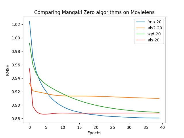
github.com/jilljenn/vae ::: ::: {.column}

See more benchmarks on \href{https://github.com/mangaki/zero}{github.com/mangaki/zero} ::: ::::::